Spreadsheet App
You can use the Spreadsheet app to input values and formulas into cells, and perform spreadsheet calculations. You can also enter statistical data into cells, perform statistical calculations, and draw statistical graphs.
Note
The maximum file size supported by the Spreadsheet app is about 30KB. The spreadsheet in this app has 999 rows and 26 columns, but due to file size restrictions, it may not be possible to input data into all of the cells. The maximum file size also depends on the type of data being input into the spreadsheet and its formatting, and on the amount of space available in main memory.
The Spreadsheet app does not support input of complex numbers.
Using the Spreadsheet Tab
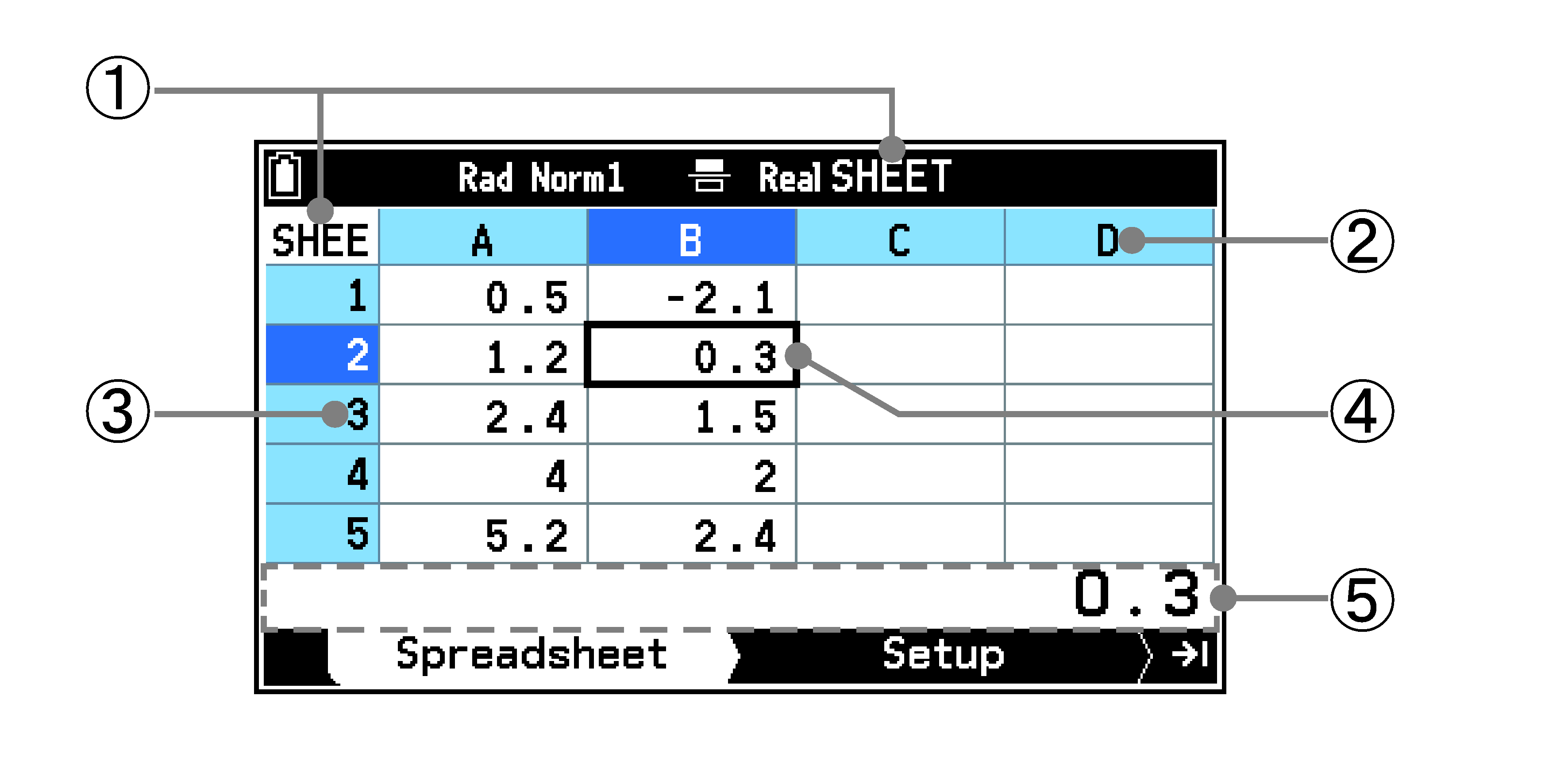
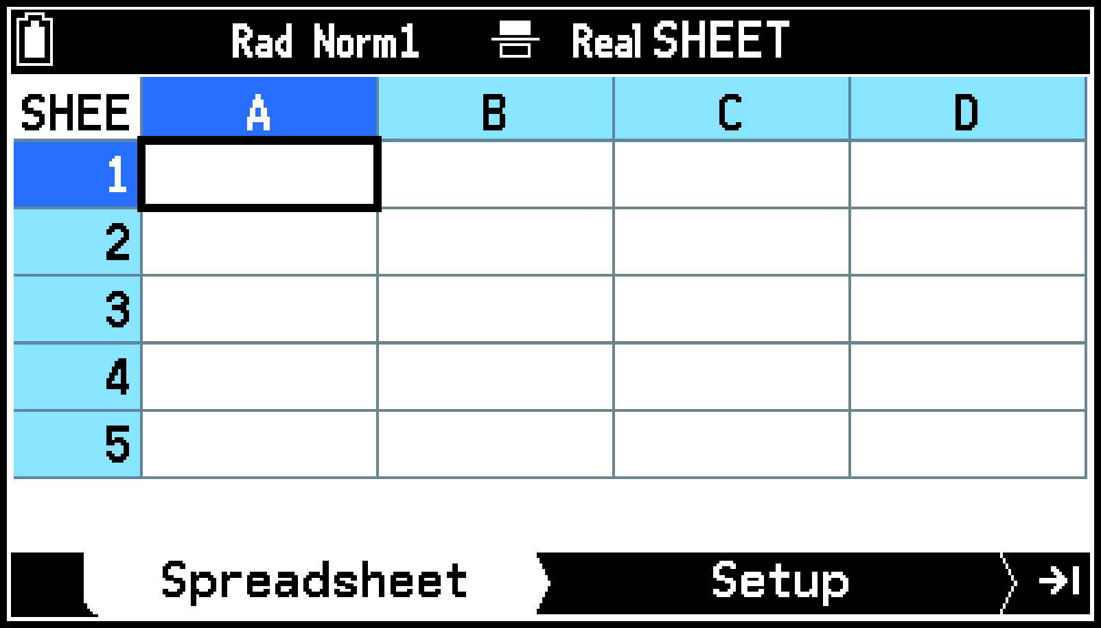
Selecting h > Spreadsheet to start up the app causes the Spreadsheet tab to appear first. The table below describes the name and function of each part of this tab.
|
① |
File name |
This is the file name of the currently opened file. “SHEET” is the initial default file of the Spreadsheet app, a “SHEET” file is automatically created when you start up the Spreadsheet app for the first time. |
|
② |
Column letter (A to Z) |
These letters and numbers indicate the current cursor position. For example, “B2” indicates the second row of column B. The row number and column letter of the currently selected cell are displayed in white with a blue background. |
|
③ |
Row number (1 to 999) |
|
|
④ |
Cursor |
The currently selected cell is indicated by a thick frame. When multiple cells are selected, all of the selected cells are enclosed in a thick frame. |
|
⑤ |
Edit box |
When a single cell is selected, the edit box shows the content of the selected cell. When multiple cells are selected, the edit box shows the range of cells that are selected. |
Selecting Cells
Before performing any operation on a cell, you must first select it. You can select a single cell, a range of cells, all the cells in a row or column, or all of the cells in the spreadsheet.
|
To select this: |
Do this: |
|---|---|
|
A single cell |
Use the cursor keys to move the cursor to the cell you want, or use the Jump command to jump directly to the cell. |
|
A range of cells |
You could select an entire row or column of cells as the start point, if you want. This changes the cursor to a double frame boundary instead of the normal thick frame. The edit box shows the range of the selected cells. To cancel cell selection, press b. |
|
An entire row of cells |
Move the cursor to column A of the row whose cells you want to select and then press l. This causes the cursor to move to the row header and selects that entire row. |
|
An entire column of cells |
Move the cursor to row 1 of the column whose cells you want to select and then press u. This causes the cursor to move to the column header and selects that entire column. |
|
All of the cells in the spreadsheet |
Press l while the entire column A is selected or press u while the entire row 1 is selected. |
Pressing s0($) while you are editing the contents of a cell with the edit box will execute a range specification operation for copying or cutting the characters in the edit box. For more information, see Copying, Cutting, and Pasting Expressions.
To use the Jump command to move the cursor
|
To move the cursor to this cell |
Do this: |
|---|---|
|
A specific cell |
|
|
Top row of current column |
Select T > [Edit] > [Jump] > [Move to the Top Row]. |
|
Column A of current row |
Select T > [Edit] > [Jump] > [Move to the First Column]. |
|
Bottom row of current column |
Select T > [Edit] > [Jump] > [Move to the Bottom Row]. |
|
Column Z of current row |
Select T > [Edit] > [Jump] > [Move to the Last Column]. |
Inputting Data into a Cell
You can input the types of data described below into a cell.
Constants:
A constant is something whose value is fixed as soon as you finalize its input. A constant can be either a numeric value or a calculation formula (such as 7+3, sin(30), A1 × 2, etc.) that does not have an equal sign (=) in front of it. A constant you input is aligned to the right of the cell.
Formula:
A formula that starts with an equal sign (=), such as =A1 × 2, is executed as it is written. The result of a formula you input is aligned to the right of the cell.
Text:
A character string that starts with a quote mark (") is treated as text. Text you input is aligned to the left of the cell. In addition, a thick vertical line is displayed on the left side of a cell when it contains text. If a cell contains the text "B, for example, its content is displayed as  .
.
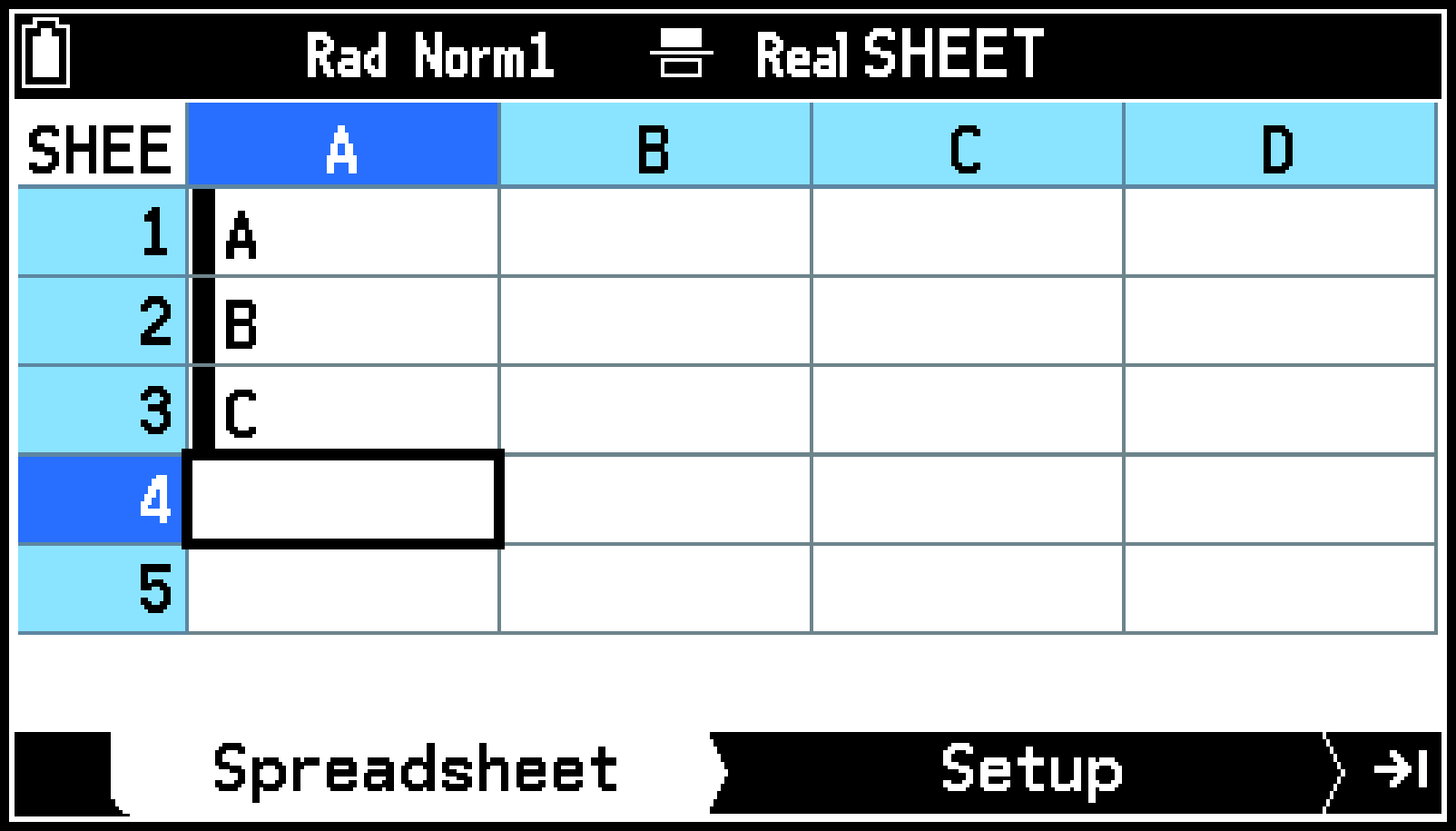
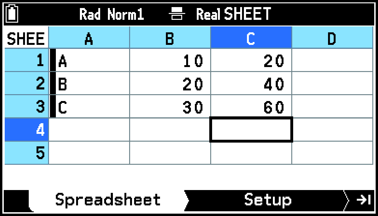
Example: Input the text A, B, C into cells A1, A2, A3, the constants 10, 10+10, 10 × 3 into cells B1, B2, B3, and formulas that specify doubling of the value in the cell to the left into cells C1, C2, C3
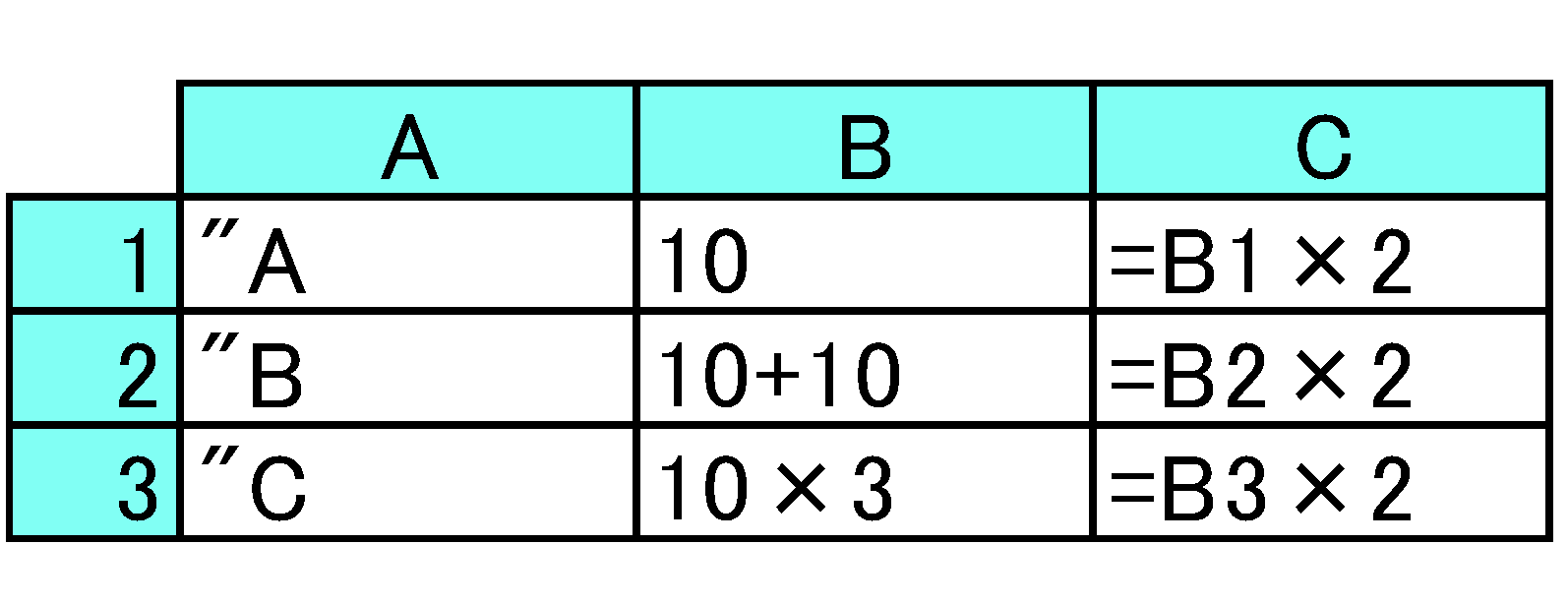
Cell contents
Display screen after input
-
h > Spreadsheet
-
Enter the text into cells A1, A2, A3.
-
Enter the constants into cells B1, B2, B3.
-
Input the formula into cell C1.
-
Copy the formula in cell C1 and then paste it into cells C2 and C3.
This displays the Spreadsheet tab.
Pk(”)PX(A)E
Pk(”)Pe(B)E
Pk(”)Pj(C)E
Ur (Moves to cell B1.)
10E
10+10E
10/3E
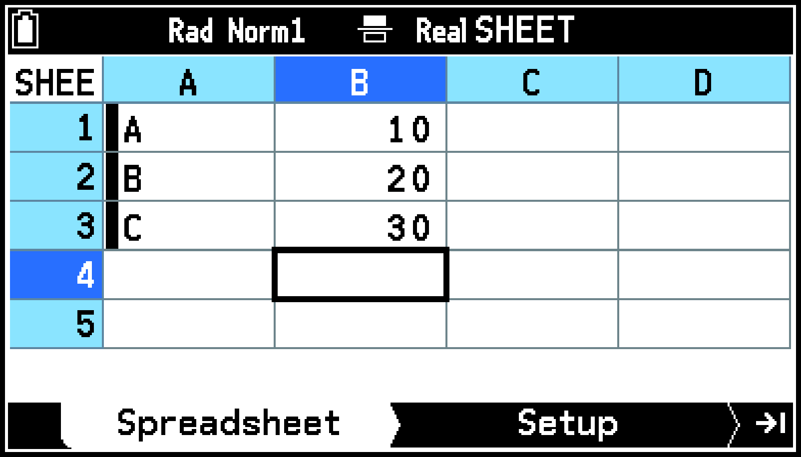
This causes the calculation results to appear in cells B2 and B3.
Ur (Moves to cell C1.)
s((=)Pe(B)1/2E
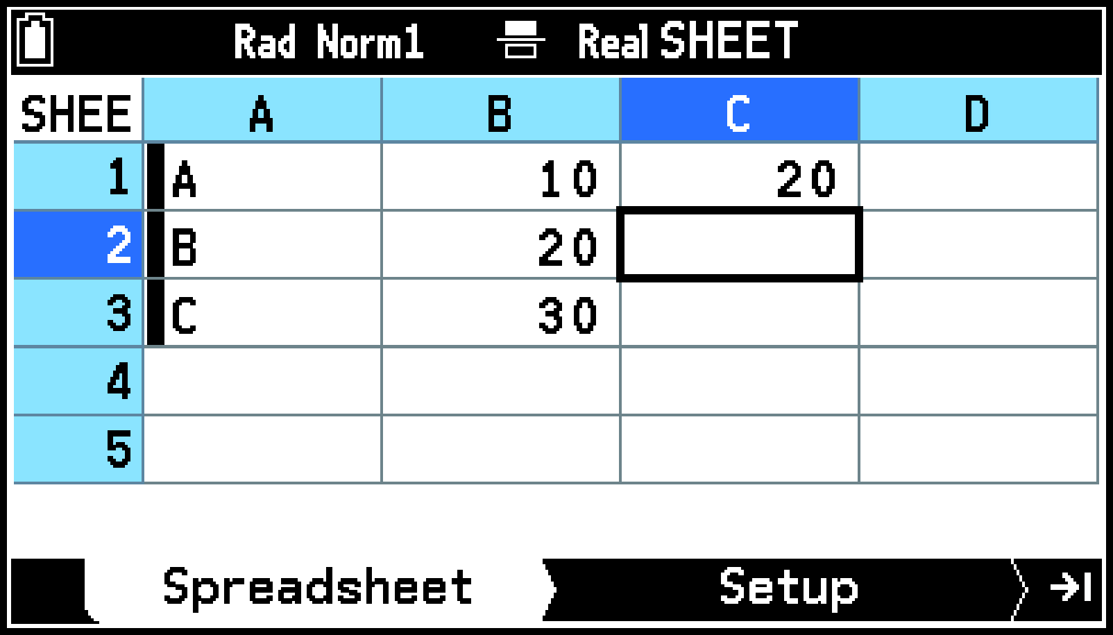
Input the formula as-is into cell C1. This causes the numeric result of the calculation to appear in the cell.
U (Moves to cell C1.)
T > [Copy & Paste] (Copies the formula in cell C1.)
dO (Pastes into cell C2.)
O (Pastes into cell C3.)
b (Cancels the copy operation.)

For details about copy and paste operations, see Copying or Cutting Cell Contents and Pasting Them in Another Location.
Note
Pressing E in steps 2 through 4 or O in step 5 above causes the cursor to move down to the next cell. You configure a setting to have the cursor move to the next cell to the right, if you want. For details, see S > [Cursor Moves] under Spreadsheet App Settings Menu Items.
If you input a letter from A to Z, or the characters r or θ as a constant or as part of a formula instead of text, it will be treated as an alpha variable. For example, if you enter PX(A)E into a cell, the letter A is treated as a constant and the value stored in variable A appears in the cell.
To fill a range of cells with the same formula (Fill)
Use the Fill command when you want to input the same formula into a specified range of cells. The rules governing relative and absolute cell name references are the same as those for copy and paste. When you need to input the same formula into cells B1, B2, and B3, for example, the Fill command lets you do so by inputting the formula once, into cell B1.
Example: To input into the range of cells B1:B3 a formula that doubles the value in the cell to the left
-
Select the range of cells where you want to input the same formula.
-
Select T > [Fill].
-
Highlight the Formula row and then input the formula you want (“=A1×2” here) into the cell at the top of the selected range (B1 here).
-
If you did not choose a cell range in step 1, specify the cell range here.
-
Highlight Cell Range.
-
Pe(B)1s`(:)Pe(B)3E
-
Select
 and then press O.
You could skip this step and start with step 2, below.
This displays the Fill screen.
s((=)PX(A)1/2E
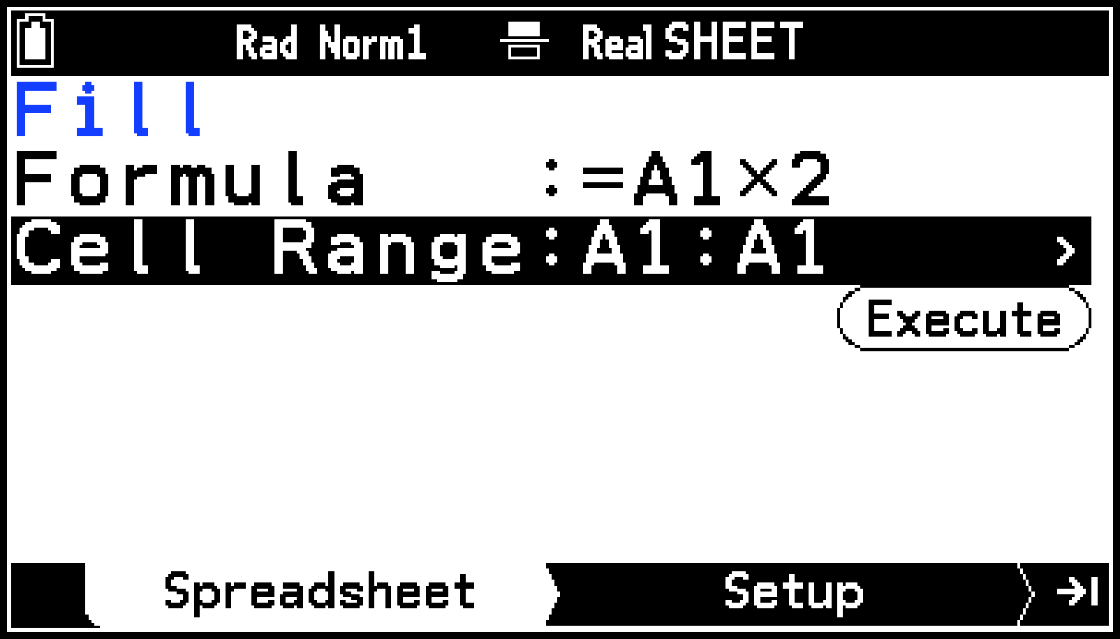
This inputs the formula into the range of cells you specified.
To fill a column of cells with a numeric sequence (Sequence)
Example: To input the sequence of numbers produced when variable X in function expression “” is assigned a value of 2 to 10 in increments of 2 into column B, starting from cell B1
-
Select the cell from which you want input of the numeric sequence to start.
-
Select T > [Sequence].
-
Configure the Sequence operation as described below.
-
After everything is the way you want, select
and then press O.
You could skip this step and start with step 2, below.
This displays the Sequence screen.
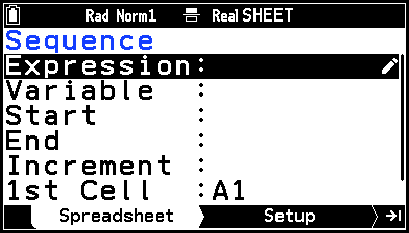
|
Parameter |
Description |
|---|---|
|
Expression |
Input the function expression for generating the number sequence. |
|
Variable |
Specify the variable name used in the function expression input for Expression. |
|
Start/End |
Specify the starting/ending value being assigned to the variable specified by Variable. |
|
Increment |
Specify the value that should be added to the variable value with each step. |
|
1st Cell |
Specify the starting cell from which the results of the function expression should be inserted. |
Xi+1E
XE2E10E2E
Pe(B)1E
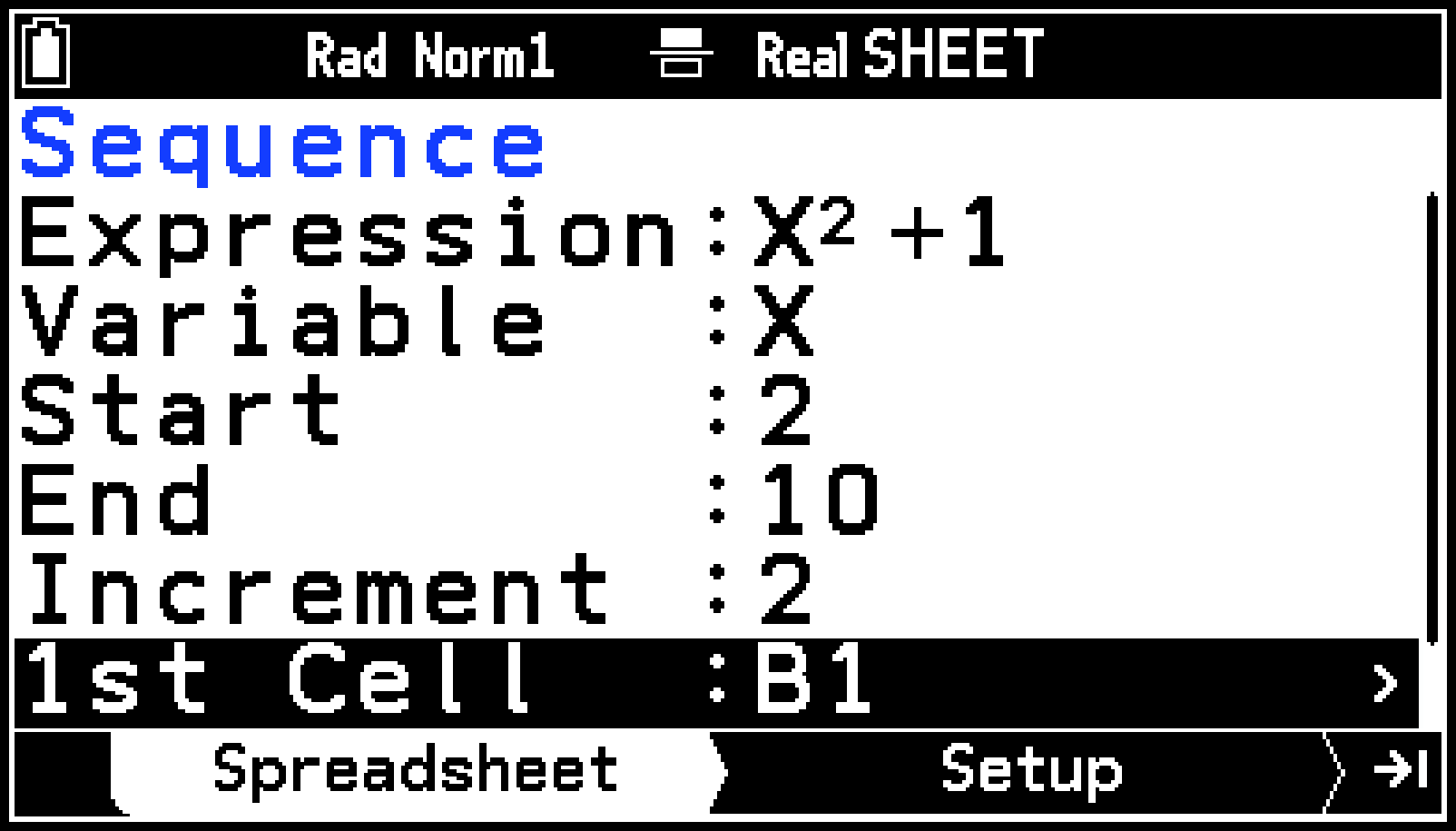
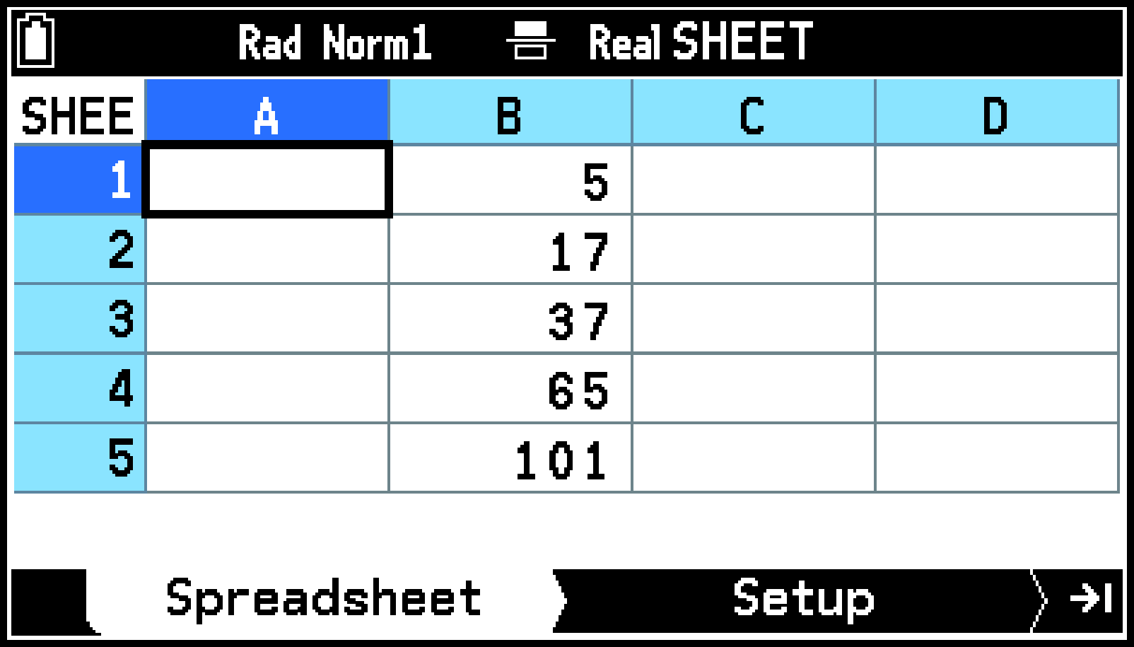
Performing the next step inputs the number sequence automatically starting from the specified cell. If any cell that is within the range of cells where the number sequence values will be input already contains data, the existing data is replaced with the number sequence values.
This performs all the required calculations according to your settings and inserts the results into the spreadsheet.
Copying or Cutting Cell Contents and Pasting Them in Another Location
Use the procedures below to copy or cut the contents of one cell or multiple cells, and then paste them into another cell or cells.
For information about what happens when you copy or cut cell contents that include cell references and paste them into another location, see Relative Cell Reference and Absolute Cell Reference.
To copy the contents of a single cell and paste them into another cell
-
Select the cell whose contents you want to copy.
-
Select T > [Copy & Paste].
-
Move the cursor to the cell where you want to paste the contents.
-
Press O.
-
If you want to paste the same contents to another cell, repeat steps 3 and 4.
-
To end the paste operation, press b.
This causes “[OK]: Paste” to appear in the status bar. You can continue to paste while this message is displayed.
The contents of the cell you copied are pasted and the cursor moves down* to the next cell.
If you want to continue pasting to the cell to which the cursor has been moved, just repeat the operation in step 4.
Default setting. The direction of cell movement is in accordance with the S > [Cursor Moves] setting.
To copy the contents of a range of cells and paste them into another location in the spreadsheet
-
Select the range of cells whose contents you want to copy.
-
Select T > [Copy & Paste].
-
Move the cursor to the cell that is the upper left corner of the range of paste destination cells.
-
Press O.
-
If you want to paste the same contents to another location, repeat steps 3 and 4.
-
To end the paste operation, press b.
This causes “[OK]: Paste” to appear in the status bar. You can continue to paste while this message is displayed.
This pastes the contents of the range of cells you copied.
To cut the contents of a single cell and paste them into another cell
-
Select the cell whose contents you want to cut.
-
Select T > [Cut & Paste].
-
Move the cursor to the cell where you want to paste, and then press O.
This causes “[OK]: Paste” to appear in the status bar.
This pastes the contents you cut. At the same time, the contents are deleted from the cell where you performed the cut operation.
To cut the contents of a range of cells and paste them into another location in the spreadsheet
-
Select the range of cells whose contents you want to cut.
-
Select T > [Cut & Paste].
-
Move the cursor to the cell that is the upper left corner of the range of paste destination cells.
-
Press O.
This causes “[OK]: Paste” to appear in the status bar.
This pastes the contents of the range of cells that you cut. At the same time, the contents are deleted from the cell where you performed the cut operation.
Note
Even if S > [Auto Recalculation] is turned off, cutting and pasting cell contents results in only the formulas in the pasted cell(s) being recalculated.
Inputting a Cell Reference
A cell reference is a symbol that references the value of one cell for use by another cell. If you input “= A1 + B1” into cell C2, for example, the spreadsheet adds the current value of cell A1 to the current value of cell B1, and displays the result in cell C2.
There are two types of cell references: relative and absolute.
Relative Cell Reference
A relative cell reference changes according to its location on the spreadsheet. The cell reference “= A1” in cell C2, for example, is a reference to the cell located “two columns to the left and one cell up” from the current cell (C2, in this case). Because of this, if we copy the contents of cell C2 and paste them into cell D12, for example, the cell reference changes automatically to “= B11”, because B11 is two columns to the left and one cell up from cell D12. Be sure to remember that relative cell references always change dynamically in this way whenever you move them using copy and paste.
Absolute Cell Reference
An absolute cell reference does not change, regardless of where it is located or where it is copied to or moved to. You can make both the row and column of a cell reference absolute, or you can make only the row or only the column of a cell reference absolute, as described below.
|
This cell reference: |
Does this: |
|---|---|
|
$A$1 |
Always refers to column A, row 1. |
|
$A1 |
Always refers to column A, but the row changes dynamically when moved, as with a relative cell reference. |
|
A$1 |
Always refers to row 1, but the column changes dynamically when moved, as with a relative cell reference. |
Let’s say, for example, that a reference to cell A1 is in cell C1. The following shows what each of the above cell references would become if the contents of cell C1 were copied to cell D12.
$A$1 → $A$1
$A1 → $A12
A$1 → B$1
Note
If the result of a copy-and-paste operation causes a relative cell reference name to change to something that is outside the range of the spreadsheet cells, the applicable column letter and/or row number is replaced by a question mark (?), and “ERROR” is displayed as the cell’s data.
To input a cell reference name using direct input
For example, to input “= A1+5” into cell B1, move the cursor to cell B1 and perform the operation below.
s((=)PX(A)1+5E
To input the absolute cell reference name symbol ($)
Select C > [Spreadsheet] > [$].
To input a cell reference name using the GRAB command
For example, to input “= A1+5” into cell B1, move the cursor to cell B1 and perform the operation below.
s((=)T > [Grab]l (Selects cell A1.) O+5E
Note
Selecting T > [Grab] causes “[OK]: Enter this cell’s ref” to appear in the status bar. While this message is displayed, you can use the Jump command in addition to the cursor keys to navigate between cells. To use the Jump command, press T while “[OK]: Enter this cell’s ref” is displayed. For details, see To use the Jump command to move the cursor.
Using Special Spreadsheet App Commands
The Spreadsheet app has several special commands like CellSum(), which returns the sum of a range of cells, and CellIf(,,), which specifies branching conditions. These special commands can be used inside of formulas.
To input these commands, use C > [Spreadsheet]. The commands described below are included in this menu.
CellIf(,,)
Returns Expression 1 when the equality or inequality provided as the branch condition is true, and Expression 2 when it is false.
Syntax:
CellIf(equality,expression 1,expression 2) or
CellIf(inequality,expression 1,expression 2)
Example:
=CellIf(A1>B1,A1,B1)
Returns the value of A1 when {Cell A1 value} > {Cell B1 value}. Otherwise, returns the value of B1.
CellMin()
Returns the minimum value in a specified range of cells.
Syntax:
CellMin(start cell:end cell)
Example:
=CellMin(A3:C5)
Returns the minimum value of the data in cell range A3:C5.
CellMax()
Returns the maximum value in a specified range of cells.
Syntax:
CellMax(start cell:end cell)
Example:
=CellMax(A3:C5)
Returns the maximum value of the data in cell range A3:C5.
CellMean()
Returns the mean value in a specified range of cells.
Syntax:
CellMean(start cell:end cell)
Example:
=CellMean(A3:C5)
Returns the mean value of the data in cell range A3:C5.
CellMedian()
Returns the median value in a specified range of cells.
Syntax:
CellMedian(start cell:end cell)
Example:
=CellMedian(A3:C5)
Returns the median value of the data in cell range A3:C5.
CellSum()
Returns the sum of the data in a specified range of cells.
Syntax:
CellSum(start cell:end cell)
Example:
=CellSum(A3:C5)
Returns the sum of the data in cell range A3:C5.
CellProd()
Returns the product of the data in a specified range of cells.
Syntax:
CellProd(start cell:end cell)
Example:
=CellProd(A3:C5)
Returns the product of the data in cell range A3:C5.
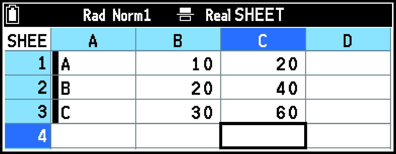
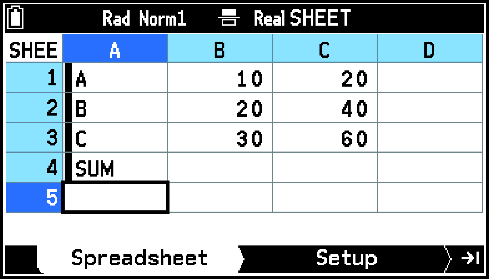
Example: To input the formula for calculating the sum the values in cells B1:B3 and C1:C3 during the example under Inputting Data into a Cell into cells B4 and C4, respectively
-
Move the cursor to cell A4 and input “SUM” as text.
-
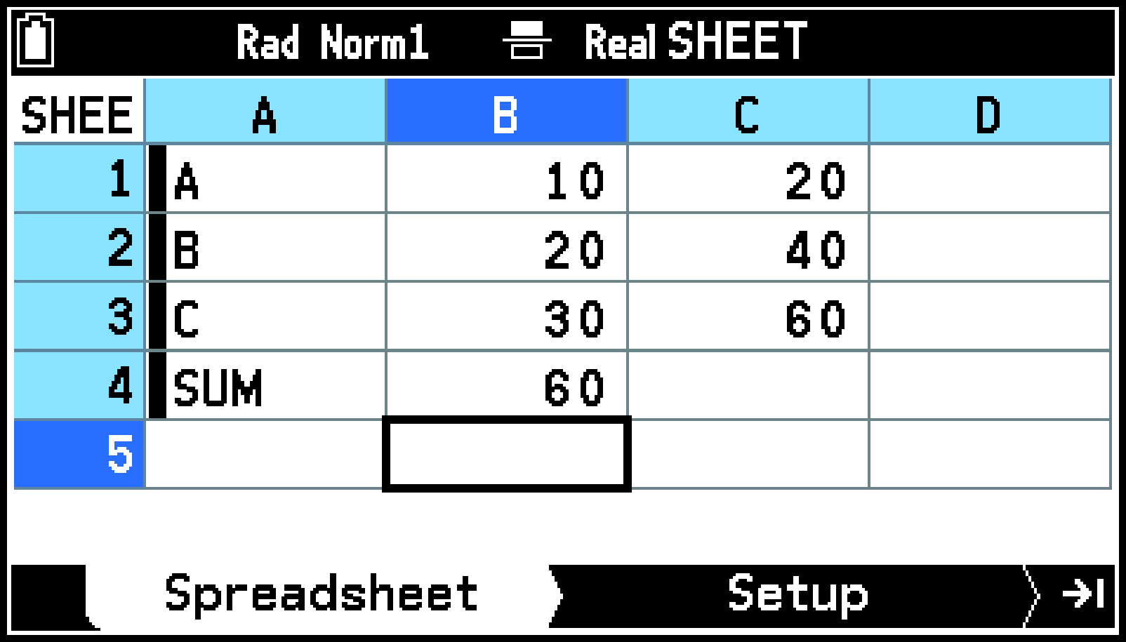
Move the cursor to cell B4 and enter the formula to calculate the sum of B1:B3.
-
Move the cursor to cell C4 and input the formula to calculate the sum of C1:C3.
Pk(”)P/(S)P1(U)P7(M)E
We want to calculate the sum of B1:B3, so we use the CellSum() command and input: =CellSum(B1:B3).
s((=)
C > [Spreadsheet] > [CellSum()]
Pe(B)1s`(:)Pe(B)3
E
s((=)
C > [Spreadsheet] > [CellSum()]
Pj(C)1s`(:)Pj(C)3
E

Editing Cell Contents
You can perform the editing operations described in the table below on the contents of individual cells, as well as on rows, columns, and the entire spreadsheet.
|
To do this: |
Perform this operation: |
||||||||
|---|---|---|---|---|---|---|---|---|---|
|
Edit the contents of a single cell |
This causes the cell contents and cursor to appear left-aligned in the edit box. |
||||||||
|
Sort data in a range of a single row or single column in ascending or descending order |
To sort in ascending order: T > [Edit] > [Sort Ascending] To sort in descending order: T > [Edit] > [Sort Descending] |
||||||||
|
Delete a row or column*1 |
You can select multiple rows or multiple columns, if you want. The row(s) or column(s) you select will be deleted. To delete row(s): T > [Delete] > [Row] To delete column(s): T > [Delete] > [Column] |
||||||||
|
Insert a row or column*2 |
You can select multiple rows or multiple columns, if you want. The row or column will be inserted at the location you selected. To insert row(s): T > [Insert] > [Row] To insert column(s): T > [Insert] > [Column] |
||||||||
|
Delete the contents of all the cells in a spreadsheet |
|
||||||||
|
Clearing the contents of selected cells |
|
This operation can also be performed using the steps below.
-
Move the cursor to the header of the row or column being deleted.
-
Select T > [Delete].
This operation can also be performed using the steps below.
-
Move the cursor to the header of the line or the column where you want to insert a line or column.
-
Select T > [Insert].
Note
A Range ERROR occurs if an insert operation causes existing cells that contain data to move outside the range of A1:Z999.
Spreadsheet File Operations
With the Spreadsheet app, you can use the file operations described in the table below.
|
To do this: |
Select this menu item: |
|---|---|
|
Close the currently open file and create a new file |
T > [File] > [New]*1 |
|
Close the currently open file and open another file |
T > [File] > [Open] |
|
Save the currently open file under a different name |
T > [File] > [Save As] |
|
Delete a file |
T > [File] > [Delete]*2 |
Inputting the name of an existing file in the dialog that appears opens the existing file without creating a new one.
Deleting the currently open file other than “SHEET” opens the file named “SHEET”. Deleting the currently open “SHEET” file automatically creates a new “SHEET” file.
Transferring Data between a Spreadsheet and CSV Files
You can import into a spreadsheet the contents of a CSV file that is stored in calculator memory or transferred from a computer. You also can save the contents of a spreadsheet as a CSV file. For information about the procedure for transferring data between a spreadsheet and CSV files, see Using CSV Files.
Specifying the Text Color and Fill Color of Each Cell
For each cell, you can specify the text color, fill color, and fill color intensity (Normal or Lighter).
To specify the text color and fill color of each cell
-
Select the range of cells whose text color and fill color you want to specify.
-
Select T > [Color].
-
Configure the above dialog box with the following settings.
-
To apply the settings you configure, press b.
|
To specify this: |
Perform this operation: |
|---|---|
|
Specify the text color |
Select [Char Color]. On the menu that appears, select the desired color. |
|
Specify the cell color |
Select [Area Color]. On the menu that appears, select the desired color. |
|
Specify the intensity of the cell color |
Select [Paint Style]. On the menu that appears, select [Normal] or [Lighter]. |
Saving Data to/Recalling Data from Variables
Spreadsheet data can be saved to variables, and data stored in variables can be recalled into a spreadsheet. Variables that can be saved to or recalled from are described below.
Save only: alpha variables
Save and recall: vector variables, matrix variables, list variables, list files*
A list file is equivalent to 26 list variables. For details, see List Files.
To save spreadsheet data to a variable
-
Select a single cell or a range of cells containing the data you want to save to a variable.
-
Select T > [Memory] > [Store].
-
On the menu that appears, select the type of variable to which you want to save the data.
-
Use the screen that appears to specify the cell range and the destination variable.
-
Select
and then press O.
Select the cell range in the table below that corresponds to the type of variable you are saving to.
|
To save to this type of variable: |
Select this range: |
|---|---|
|
Alpha variable |
Single cell |
|
List variable or vector variable |
A range of cells in a single row or a single column |
|
List file or matrix variable |
A range of cells that spans multiple rows and columns |
You could skip this step and start with step 2, below.
|
To save to this type of variable: |
Select this menu item: |
Destination: |
|---|---|---|
|
Alpha variable |
[Alpha] |
A to Z, r, or θ |
|
List variable |
[List] |
List 1 to List 26 |
|
List file |
[File] |
File 1 to File 6 |
|
Matrix variable |
[Matrix] |
Mat A to Mat Z |
|
Vector variable |
[Vector] |
Vct A to Vct Z |
If you specified a cell range in step 1 of this procedure, you do not need to specify it again here.
Refer to “Destination” in the table in step 3 for the destinations that you can specify.
Note
Text color and other formatting settings are disregarded when cells are saved to a variable.
The following describes what happens if you try to store data in a variable when a cell does not contain any data, when a cell contains text, or when ERROR is displayed for a cell.
If you are assigning data to an alpha variable, an error occurs.
If you are storing data in a list variable, a list file, a matrix variable, or a vector variable, 0 is written into the applicable cell(s).
To recall data stored in a variable into a spreadsheet
-
Specify the cell to which you want to recall the variable data.
-
Select T > [Memory] > [Recall].
-
On the menu that appears, choose the type of variable whose data you want to recall.
-
Use the screen that appears to specify the variable being recalled and the destination cell.
-
Select
and then press O.
Select a cell for recall in accordance with the type of variable as shown in the table below.
|
To recall from this type of variable: |
Select a cell like this: |
|---|---|
|
List variable |
When “Down” is selected for S > [Cursor Moves]: Select the cell at the top of the range to which you want to recall data. The data is recalled from top to bottom starting from the selected cell. When “Right” is selected for S > [Cursor Moves]: Select the leftmost cell of the range to which you want to recall data. The data is recalled from left to right starting from the selected cell. |
|
List file or matrix variable |
Select the cell at the top-left corner of the range to which you want to recall data. |
|
Vector variable |
Select the leftmost cell (for a vector with 1 row and n columns) or the topmost cell (for a vector with n rows and 1 column) of the range to which you want to recall data. |
You could skip this step and start with step 2, below.
|
To recall from this type of variable: |
Select this menu item: |
Recall source: |
|---|---|---|
|
List variable |
[List] |
List 1 to List 26 |
|
List file |
[File] |
File 1 to File 6 |
|
Matrix variable |
[Matrix] |
Mat A to Mat Z |
|
Vector variable |
[Vector] |
Vct A to Vct Z |
See the “Recall source” column in the table in step 3 for information about the types of variables that can be specified.
If you selected a cell in step 1 of this procedure, you do not need to specify a cell here.
Note
If you specify a cell that results in the recalled data not being able to fit within the range of the spreadsheet (A1:Z999), pressing ![]() in step 5 results in an error and does not execute the recall.
in step 5 results in an error and does not execute the recall.
The recalled data is formatted according to the default formatting of the cell to which it is recalled.
Auto Recalculation and Recalculate
“Auto Recalculation” is a setting item on the Settings menu. With the Spreadsheet app’s initial default setting (Auto Recalculation: On), all formulas in a spreadsheet are automatically re-calculated whenever you open a file or perform an editing operation in the Spreadsheet app. Depending on the content of the spreadsheet, auto re-calculation can take a long time to complete. When Auto Recalculation is disabled (Off), you need to execute re-calculation manually as required.
To execute re-calculation manually
Select T > [Recalculate].
Note
Even if the Auto Recalculation setting is On, you should execute T > [Recalculate] in the cases below.
When the Settings menu is used to change the Angle setting
When a cell contains a formula using an alpha variable or a function variable and the corresponding variable is updated
Statistical Calculations and Graph Drawing
You can perform statistical calculations and draw statistical graphs using data input into a spreadsheet.
Inputting Data
Depending on the statistical data being processed, input the data using columns 1, 2, and 3 of the Spreadsheet tab.
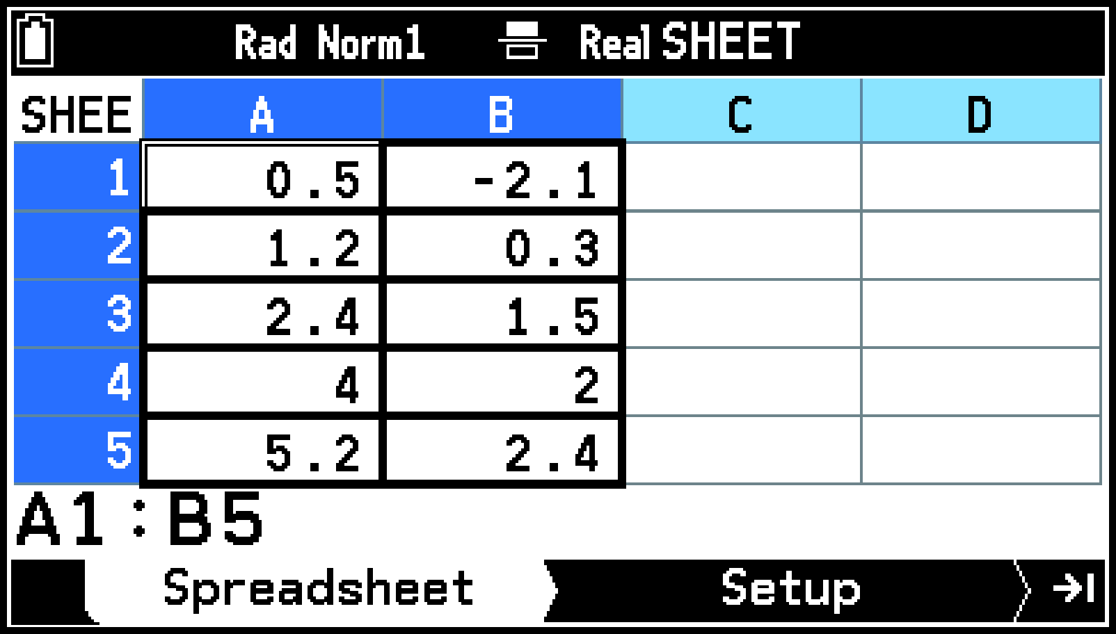
Input of 2-Variable data without frequencies
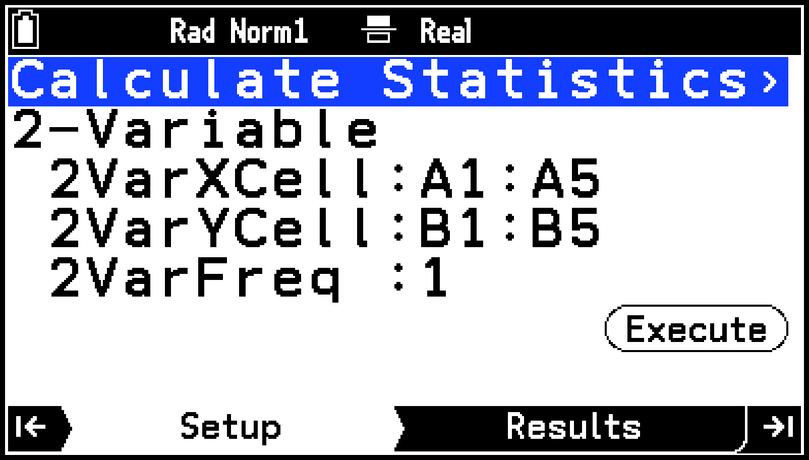
Example setup (Setup tab)
|
For this statistical data: |
Input like this: |
|---|---|
|
1-Variable (no frequencies) |
Input variable-X data (1VarXCell*1) into a single column. |
|
1-Variable (with frequencies) |
Input variable-X data (1VarXCell*1) into the first column and frequency data (1VarFreq*2) into the second column. |
|
2-Variable (no frequencies) |
Input variable-X data (2VarXCell*1) into the first column and variable-Y data (2VarYCell*1) into the second column. |
|
2-Variable (with frequencies) |
Input variable-X data (2VarXCell*1) in the first column, variable-Y data (2VarYCell*1) into the second column, and frequency data (2VarFreq*2) into the third column. |
In the Spreadsheet app Setup tab, specify the cell range for data being used for 1-Variable statistical calculation to 1VarXCell (or XCellRange), the cell range for data being used for 2-Variable statistical calculation to 2VarXCell, 2VarYCell (or XCellRange, YCellRange).
In the Spreadsheet app Setup tab, the cell range of frequency data used for 1-Variable statistical calculation is displayed as 1VarFreq (or Frequency), while the cell range of frequency data used for 2-Variable statistical calculation is displayed as 2VarFreq (or Frequency).
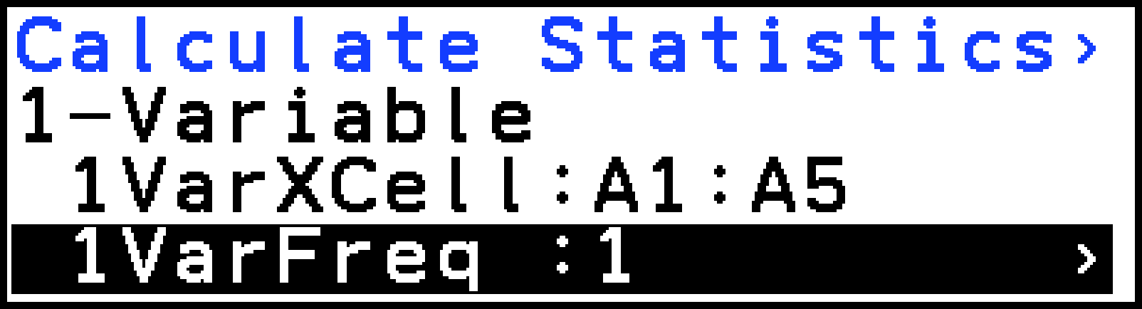
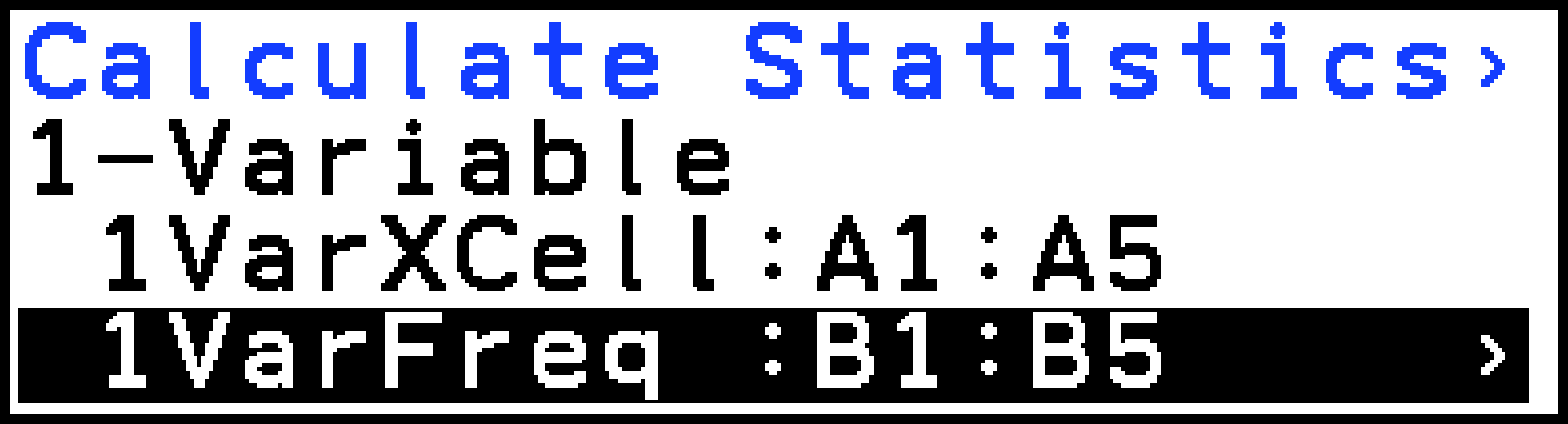
Frequencies
There are two ways to input statistical data: with frequencies and without frequencies (1 is used for all data frequencies). You can specify which method you want to use on the Setup tab that appears when you press > on the Spreadsheet tab, as shown in the example below.
 |
 |
|
Using cell range A1:A5 as data |
Using cell range A1:A5 as data |
Important!
The values contained in the cell range used as the frequency data should be 0 or positive values only. Even a single negative value causes an error (Out of Domain).
Statistical data with a frequency of 0 is not used for calculation of minimum and maximum values.
Displaying Summary Statistics or Regression Model Information
You can use the procedure below to find and display various summary statistics from 1-Variable or 2-Variable statistical data. This procedure can also be used to display regression equation coefficients and coefficients of determination (referred to as “regression model information” in this manual) when regression models are applied to 2-Variable statistical data.
To display summary statistics or regression model information
-
Input the statistical data to use in the calculation.
-
Select the range of cells into which you input statistical calculation data.
-
Press >.
-
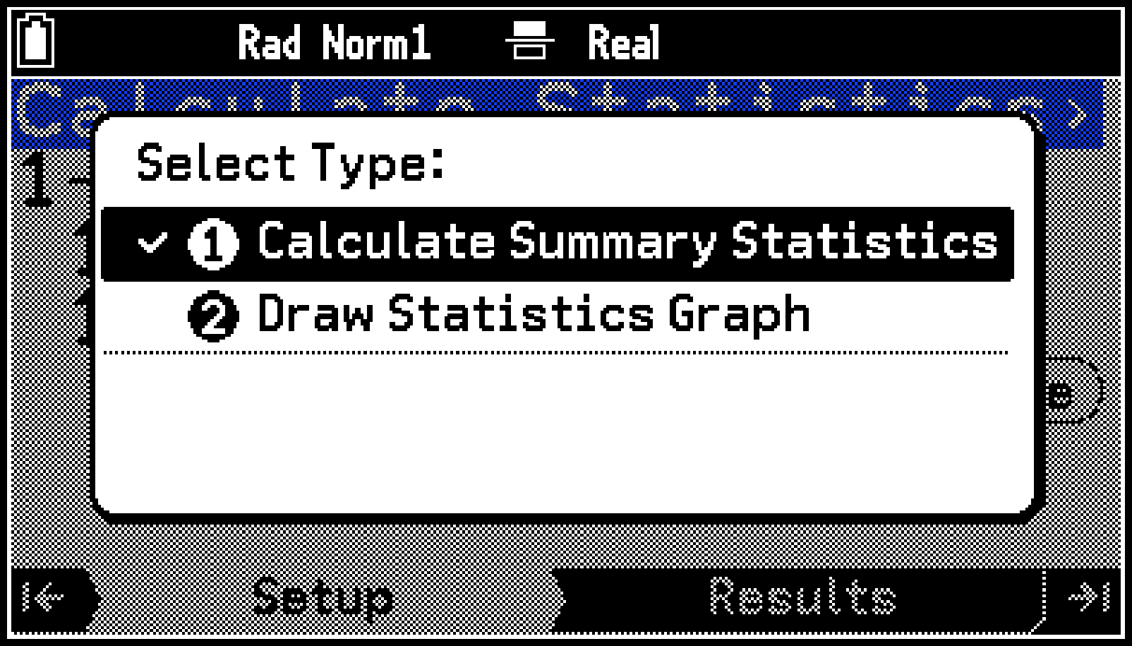
Highlight the first line of the Setup tab and then press O.
-
Select [Calculate Summary Statistics].
-
Highlight line 2 on the tab and then press O.
-
On the menu that appears, select the type of statistical calculation you want to perform.
-
Specify the cell range containing the statistical data being used in the calculation as required.
-
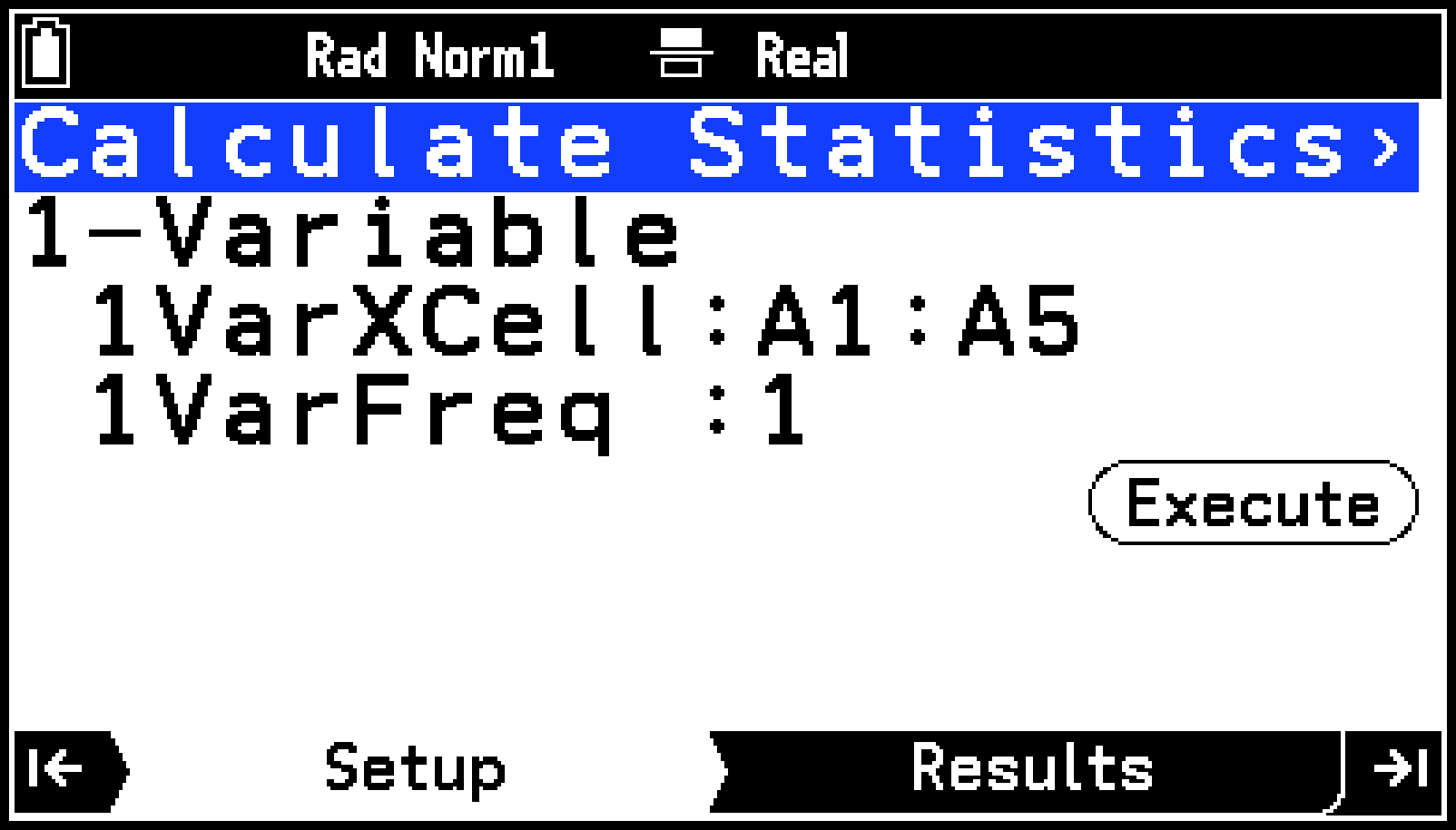
Highlight [1VarXCell] and then press O.
-
Use the dialog box that appears to input the range of X-data cells and then press O.
-
Highlight [1VarFreq] and then press O.
-
If you do not want to use frequency data, select [1] on the menu.
If you want to use frequency data, select [Cell Range] and then advance to step (5). -
Use the dialog box that appears to input the range of frequency data cells and then press O.
-
Highlight [2VarXCell] and then press O.
-
Use the dialog box that appears to input the range of X-data cells and then press O.
-
Highlight [2VarYCell] and then press O.
-
Use the dialog box that appears to input the Y-data cell range and then press O.
-
Highlight [2VarFreq] and then press O.
-
If you do not want to use frequency data, select [1] on the menu.
If you want to use frequency data, select [Cell Range] and then advance to step (7). -
Use the dialog box that appears to input the range of frequency data cells and then press O.
-
Press >. Or highlight
and then press O.
For details, see Inputting Data.
You could skip this step and go to step 3, below.
If this causes the Select Type menu to appear, go to step 5 of this procedure. Otherwise, go to step 4.
This causes the Calculate Statistics menu to appear on the Setup tab.
|
To do this: |
Select this menu item: |
|---|---|
|
Display summary statistics based on 1-Variable statistical data (X) |
1-Variable |
|
Display summary statistics based on 2-Variable statistical data (X, Y) |
2-Variable |
|
Display regression model information based on 2-Variable statistical data (X, Y) |
Linear Regression(a+b) |
|
Linear Regression(a+b) |
|
|
Med-Med Regression |
|
|
Quadratic Regression |
|
|
Cubic Regression |
|
|
Quartic Regression |
|
|
Logarithm Regression |
|
|
Exp Regression(a・e^b) |
|
|
Exp Regression(a・b^) |
|
|
Power Regression |
|
|
Sinusoidal Regression |
|
|
Logistic Regression |
For 1-Variable statistical data:
For 2-Variable statistical data:
This displays the summary statistics or regression model information you selected in step 6 on the Results tab. If a scroll bar appears along the right edge of the window, use d and u to scroll the display.
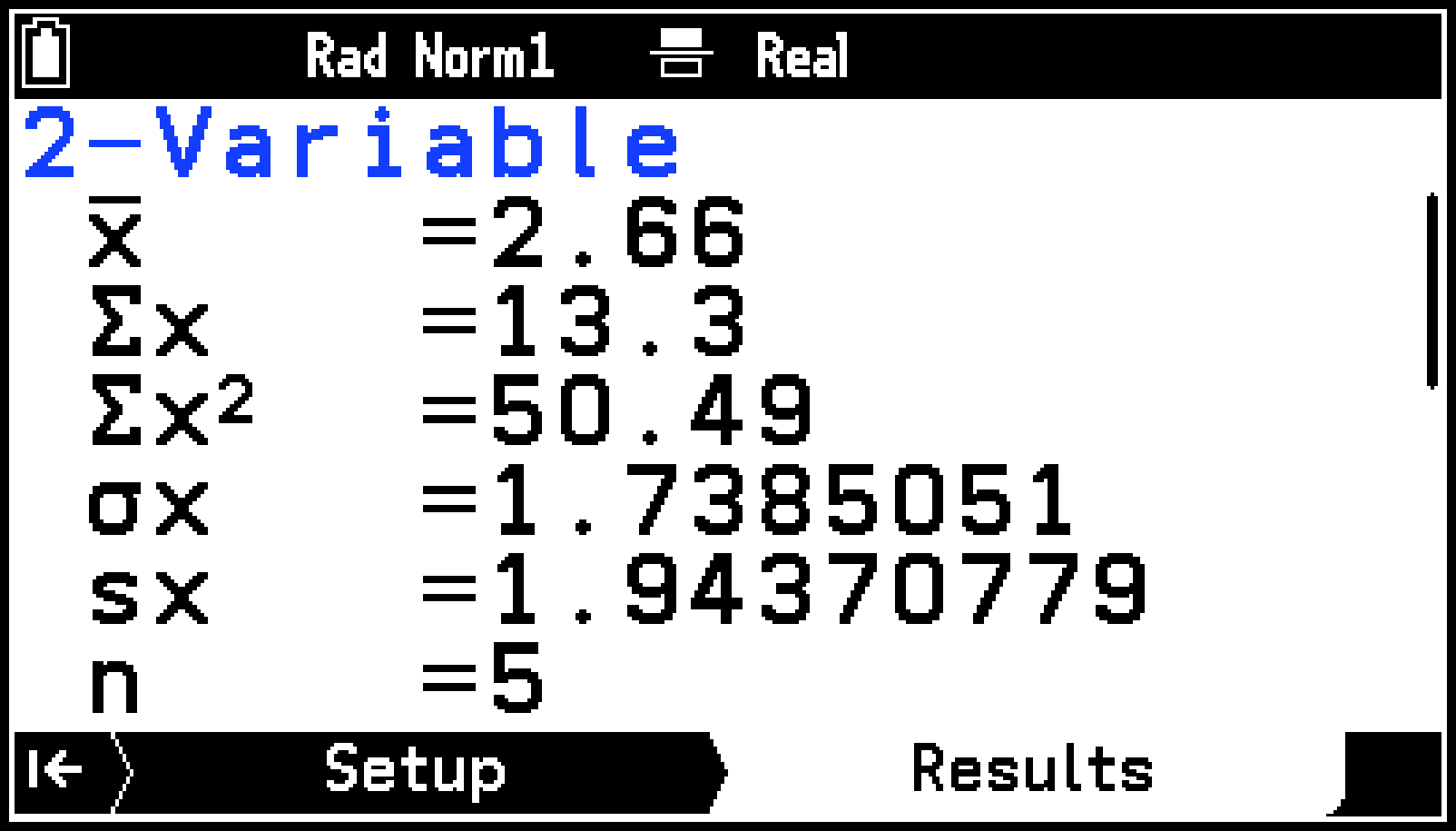
See Summary Statistics and Regression Model Information for the meanings of the values that appear on the display.
Drawing a Statistics Graph
You can use 2-Variable statistical data to draw scatter plots and various regression graphs. 1-Variable statistical data can be used to draw seven types of graphs, including histograms and box-and-whisker diagrams. After drawing a graph, you can display summary statistics and regression model information.
Drawing a 1-Variable Statistics Graph (Histogram, Box-and-Whisker Diagram, etc.)
You can perform the operations below based on 1-Variable statistical data you input into a spreadsheet.
-
Draw a Box Plot, Histogram, Broken Line Graph, Pie Chart, Bar Graph, Normal Probability Plot, or Normal Density Curve.
-
Display summary statistics after drawing the graph (except for Pie Chart).
To draw a 1-Variable statistics graph
-
Input the statistical data to use in the calculation.
-
Select the range of cells into which you input statistical calculation data.
-
Press >.
-
Highlight the first line of the Setup tab and then press O.
-
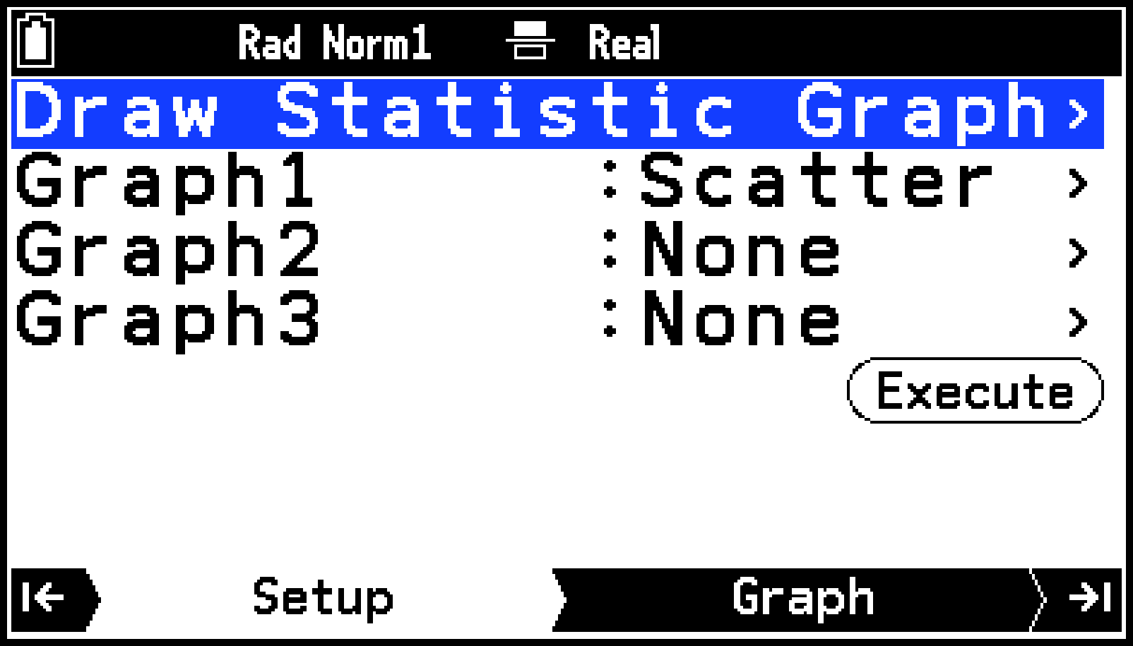
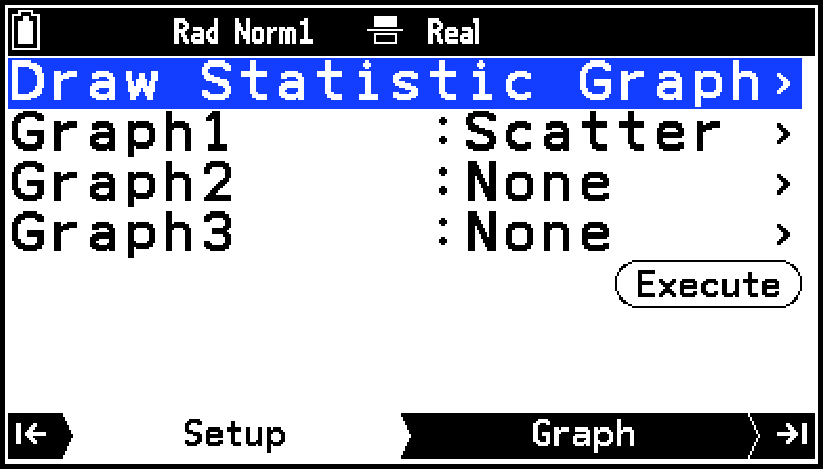
On the Select Type menu, select [Draw Statistics Graph].
-
Select the type of graph you want to draw.
-
Highlight [Graph1] and then press O.
-
Press O again.
-
Highlight the type of graph you want to draw from the menu and then press O.
-
Specify statistical data cell range on the spreadsheet.
-
Highlight [XCellRange] and then press O.
-
Use the dialog box that appears to input the range of data cells and then press O.
-
Highlight [Frequency] and then press O. (Excluding Normal Probability Plot)
-
Highlight [Category] and then press O.
-
Use the dialog box that appears to input the range of data category name cells and then press O.
-
Highlight [Data] and then press O.
-
Use the dialog box that appears to input the range of data cells and then press O.
-
Highlight [Category] and then press O.
-
Use the dialog box that appears to input the range of data category name cells and then press O.
-
Highlight [Data1] and then press O.
-
Use the dialog box that appears to input enter the range of data cells and then press O.
-
Repeat the steps (3) and (4) above for [Data2] and [Data3].
-
Specify the graph color and other settings as required.
-
To draw the graph, press >. Or highlight
and then press O. -
To view summary statistics, press >. (This operation cannot be used for a Pie Chart.)
For details, see Inputting Data.
You could skip this step and go to step 3, below.
If this causes the Select Type menu to appear, go to step 5 of this procedure. Otherwise, go to step 4.
This causes the Draw Statistics Graph menu to appear on the Setup tab.
This causes the Setup tab display to change to the Graph1 setting menu.

This displays a menu for selecting the graph type.
For a Box Plot, Histogram, Broken Line Graph, Normal Probability Plot, or Normal Density Curve:
For a Pie Chart:
For a Bar Graph:
You can specify up to three sets of data to draw a bar graph.
When specifying [Data2] and [Data3], be sure to specify the same number of rows as [Data1] data. If the number of rows is different, an error (Dimension ERROR) occurs.
When specifying two sets of data, be sure to specify the cell range for [Data1] and [Data2]. If a cell range is specified for [Data1] and [Data3] while [Data2] is set to “None”, an error (Condition ERROR) occurs.
For details, see Setting Items for Each 1-Variable Statistics Graph Type.
The graph is displayed on the Graph tab.
If the graph you selected in step 6-(3) is a Histogram or Broken Line Graph, a dialog box appears where you can specify Start (-coordinate of the graph drawing start point) and Width (graph drawing width). Input each of the values, highlight ![]() , and then press O.
, and then press O.
For information about the operations you can perform on the Graph tab, see Graph Window Operations.
This causes the summary statistics to appear on the Results tab. You can use d and u to scroll the display contents.
See Summary Statistics for the meanings of the displayed values.
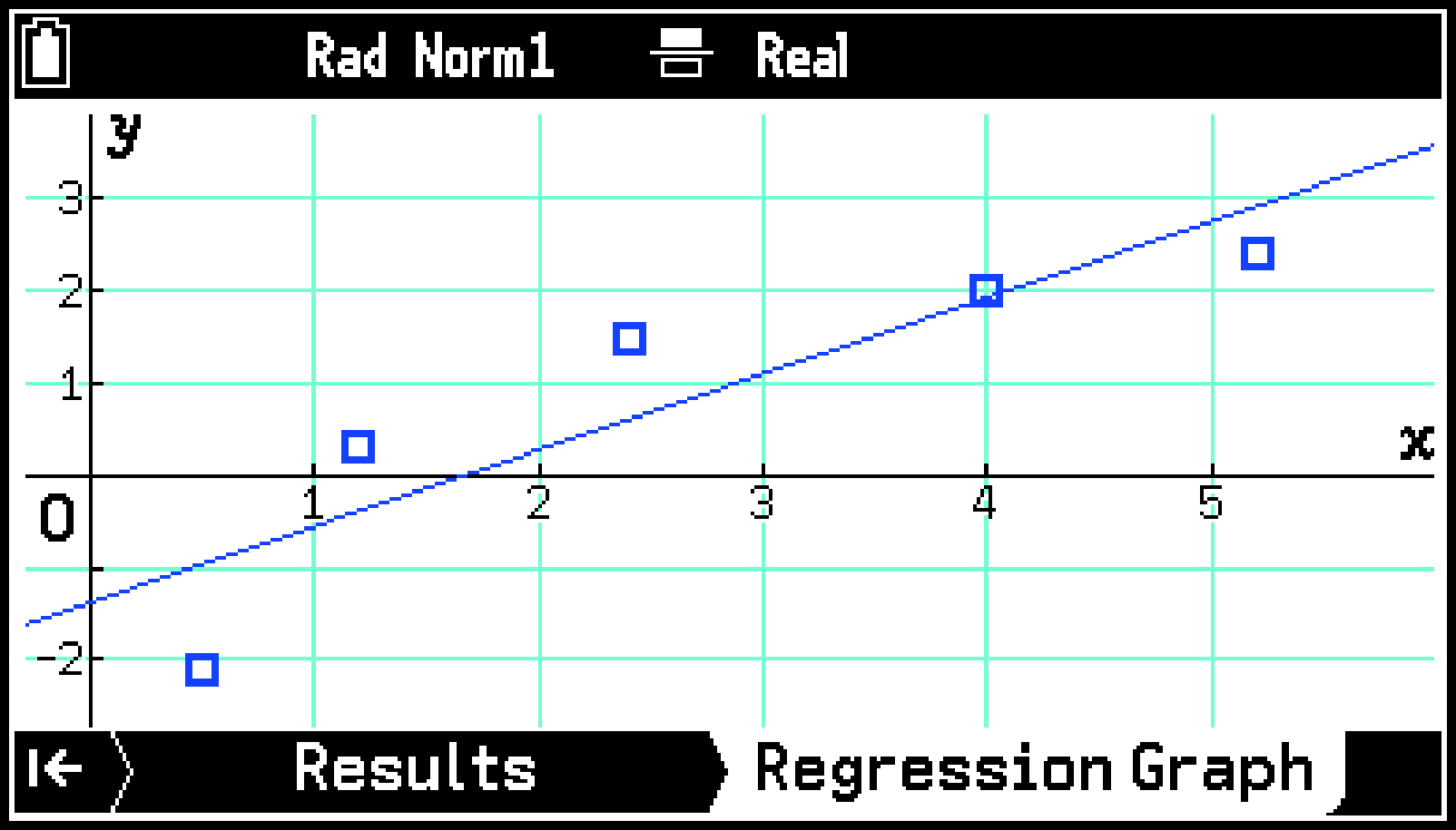
Drawing a 2-Variable Statistics Graph (scatter plot or regression graph)
You can perform the operations below based on 2-Variable statistical data.
-
Draw a Scatter Plot, xy Line Graph, or regression graph
-
After drawing a graph, display summary statistics or regression model information
-
Draw a regression graph over a graph described in (1) above*
Common practice in (1) is to draw a Scatter Plot and then draw a regression graph over it. You can also draw a regression graph over a xy Line Graph or another regression graph.
To draw a 2-Variable statistics graph
-
Input the statistical data to use in the calculation.
-
Select the range of cells into which you input statistical calculation data.
-
Press >.
-
Highlight the first line of the Setup tab and then press O.
-
On the Select Type menu, select [Draw Statistics Graph].
-
Select the type of graph you want to draw.
-
Highlight [Graph1] and then press O.
-
Press O again.
-
Highlight the type of graph you want to draw from the menu and then press O.
-
Specify statistical data cell range on the spreadsheet.
-
Highlight [XCellRange] and then press O.
-
Use the dialog that appears to input the data cell range and then press O.
-
Highlight [YCellRange] and then press O.
-
Use the dialog that appears to input the data cell range and then press O.
-
Highlight [Frequency] and then press O. (This operation does not work with a Sinusoidal Regression Graph or Logistic Regression Graph.)
-
Specify the graph color and other settings as required.
-
To draw the graph, press >. Or highlight
and then press O. -
Display summary statistics or regression model information.
-
Press >.
-
Perform the operations shown in the table below.
-
Press O.
-
Press > to go to the Regression Graph tab and draw a regression graph.
-
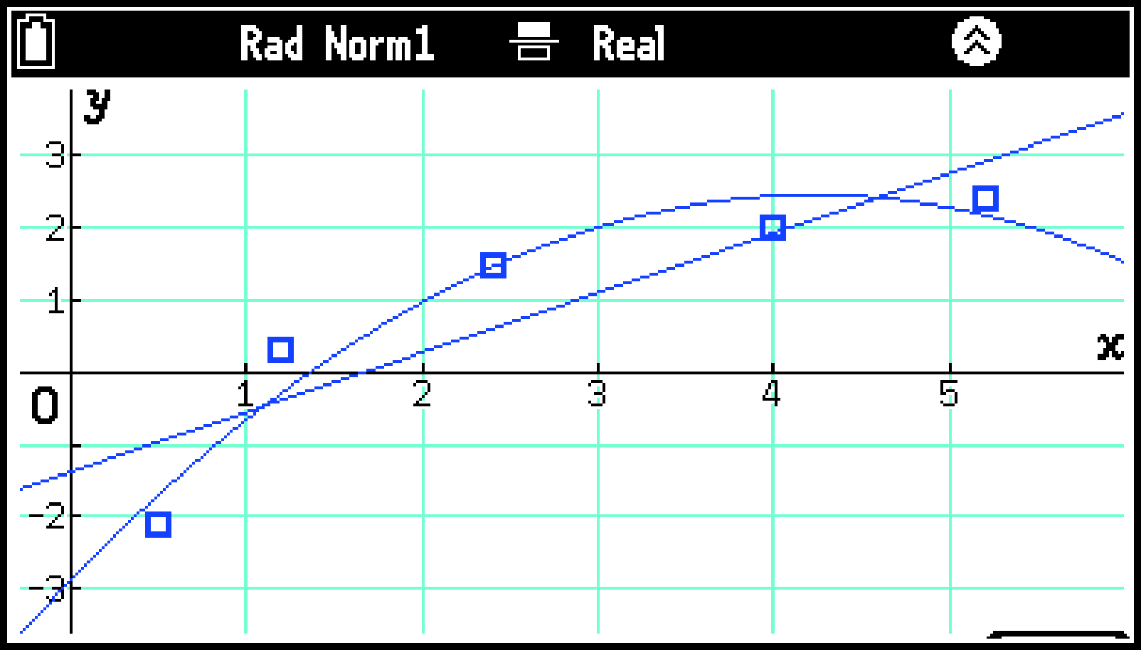
Add regression graphs as needed.
-
Select T > [Draw Regression Graph].
-
From the menu that appears, select the regression model you want and then press O.
For details, see Inputting Data.
You could skip this step and go to step 3, below.
If this causes the Select Type menu to appear, go to step 5 of this procedure. Otherwise, go to step 4.
This causes the Draw Statistics Graph menu to appear on the Setup tab.
This causes the Setup tab display to change to the Graph1 setting menu.
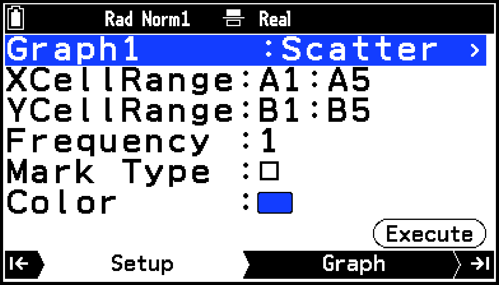
This displays a menu for selecting the graph type.
Mark Type: If you selected Scatter Plot or xy Line Graph as the graph type, specify the mark to use for the plot.
Color: Specifies the graph draw color.
The graph is displayed on the Graph tab.
For information about the operations you can perform on the Graph tab, see Graph Window Operations.
|
To display this information: |
Select this menu item: |
|---|---|
|
Summary statistics |
2-Variable |
|
Regression model information |
Linear Regression(a+b) |
|
Linear Regression(a+b) |
|
|
Med-Med Regression |
|
|
Quadratic Regression |
|
|
Cubic Regression |
|
|
Quartic Regression |
|
|
Logarithm Regression |
|
|
Exp Regression(a・e^b) |
|
|
Exp Regression(a・b^) |
|
|
Power Regression |
|
|
Sinusoidal Regression |
|
|
Logistic Regression |
This displays the details of the menu item you selected in step (2) above on the Results tab.
See Summary Statistics and Regression Model Information for the meanings of the displayed values.
Choosing one of the regression models in step 10 draws a regression graph over the graph drawn in step 9.
Choosing 2-Variable displays only the graph drawn in step 9.
You can add multiple regression graphs on the Regression Graph tab. To do this, perform the steps below.
This adds the graph of the regression model you selected.
You can repeat steps (1) and (2) above to add more regression graphs.
For operations that are available on the Regression Graph tab, see Graph Window Operations.
Note
For details about Graph1 to Graph3 on the Setup tab in step 5 above, see Drawing Graphs Using Multiple Graph Setups.
The settings of the statistics graph View Window are automatically configured according to the graph being drawn. For more information, see Statistics Graph View Window Settings.
Spreadsheet App Settings Menu Items
The Settings menu items described below are specific to the Spreadsheet app.
|
S > [Auto Recalculation] … |
Toggles between automatic recalculation and no recalculation for each data input. |
|
S > [Edit Box Shows] … |
Specifies whether the contents of a formula already entered in a cell are displayed as a formula or as a value. Even if value is specified by this setting, the formula is displayed when editing cell contents. |
|
S > [Cursor Moves] … |
Selects the cursor movement direction (down or right) after data is input or pasted into a cell. |