Statistics App
The Statistics app provides you with the tools you need to perform statistical calculations based on input data, to display summary statistics and regression model information, and to draw graphs. It also provides you with hypothesis testing and confidence interval capabilities.
Selecting What You Want to Do with the Statistics App
-
h > Statistics
-
Press >.
-
Highlight the first line of the Setup tab and then press O.
-
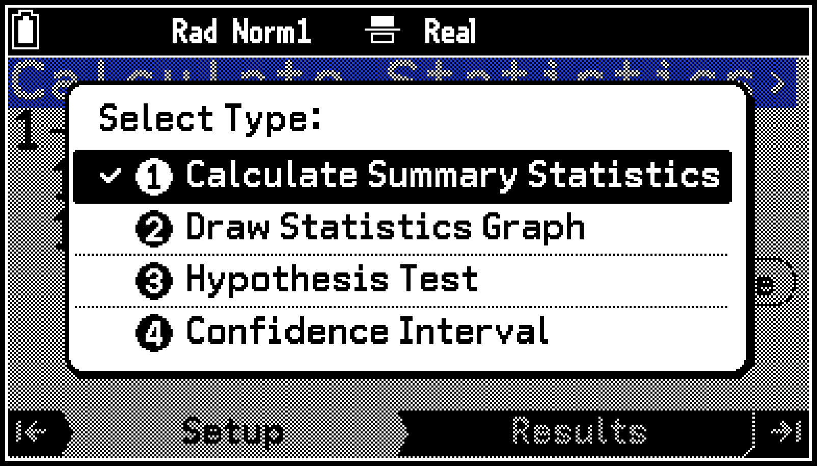
Use the menu to select what you want to do.
-
Press O.
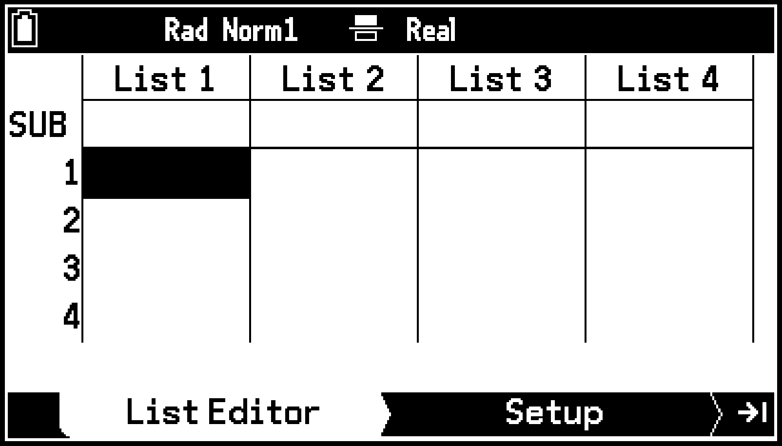
This enters the Statistics app with the List Editor tab active.
If this causes the Select Type menu to appear, go to step 4 of this procedure. Otherwise, go to step 3.
|
To do this: |
Highlight this menu item: |
|---|---|
|
Displaying Summary Statistics or Regression Model Information*1 |
[Calculate Summary Statistics] |
|
[Draw Statistics Graph] |
|
|
[Hypothesis Test] |
|
|
[Confidence Interval] |
Regression model information includes regression equations coefficients, coefficient of determination, etc.
Scatter plots and regression graphs based on 2-Variable data, histograms and box-and-whisker diagrams based on 1-Variable data, etc.
This displays on the Setup tab a menu of settings for the item you selected.
Inputting Data
The Statistics app’s List Editor is an app-specific editor for inputting and editing statistical data. You can use List Editor to create up to 26 list variables (List 1 to List 26) at a time.
Create from one to three list variables, depending on the statistical data to be processed.*1
|
Statistical data: |
Required list variable(s): |
|---|---|
|
1-Variable (no frequencies) |
One list variable to assign to XList*2 |
|
1-Variable (with frequencies) |
Two list variables to assign to XList and Freq*2 |
|
2-Variable (no frequencies) |
Two list variables to assign to XList and YList*2 |
|
2-Variable (with frequencies) |
Three list variables to assign to XList, YList and Freq*2 |
The method of statistical data creation for 1-Variable or 2-Variable statistical calculation is different from that for performing hypothesis tests or finding confidence intervals.
This calculator displays list data used for 1-Variable statistical calculations as XList, list data used for 2-Variable statistical calculations as XList and YList, and list data used for frequencies as Freq or Frequency.
Frequencies
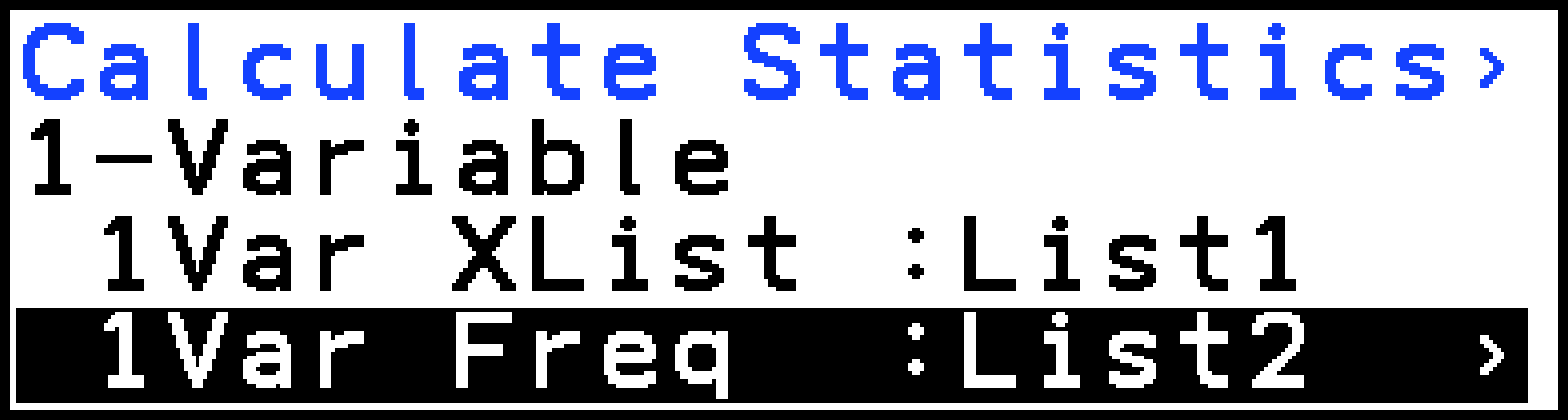
There are two ways to input statistical data: with frequencies and without frequencies (1 is used for all data frequencies). You can specify which method you want to use on the Setup tab that appears when you press > in List Editor, as shown in the example below.
 |
 |
|
Uses List1 for data. Frequency of all data values: 1 |
Uses List1 for data. Uses List2 for frequencies. |
Important!
The values contained in a frequency list should be 0 or positive values only. Even a single negative value causes an error (Out of Domain).
Statistical data with a frequency of 0 is not used for calculation of minimum and maximum values.
Inputting Data in List Editor
You can use either of the two methods below to input data in List Editor.
Individual cell input
With this method, you input a value into a cell and then press E.
You can also input a calculation into a cell. If you do, the numeric value that is the result of the calculation is entered immediately after you press E.
Batch input using the form {1,2,3,...}
Example: To input {1,2,3,4,5}
-
Use the cursor keys to highlight the name of the list you want to use.
-
Select C > [Statistics] > [{}], input the value, and then press E.
1`2`3`4`5E

Assigning Other List Variables
You can assign List 1 data directly to List 2 or assign a list calculation result to List 2.
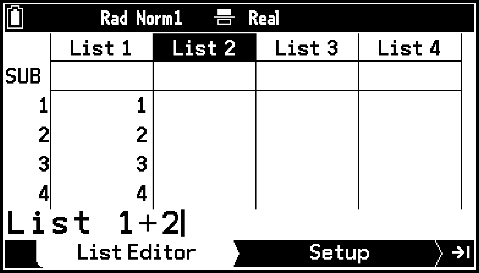
Example: To assign List 1+2 (adds 2 to each element of List 1) to List 2
-
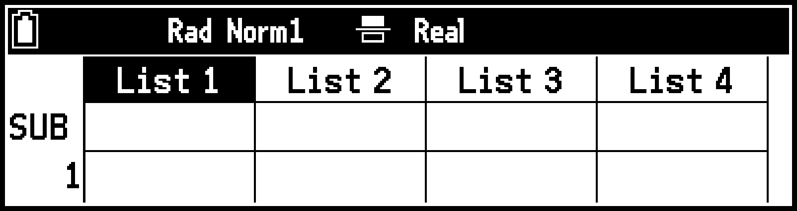
Use the cursor keys to highlight list name List 2.
-
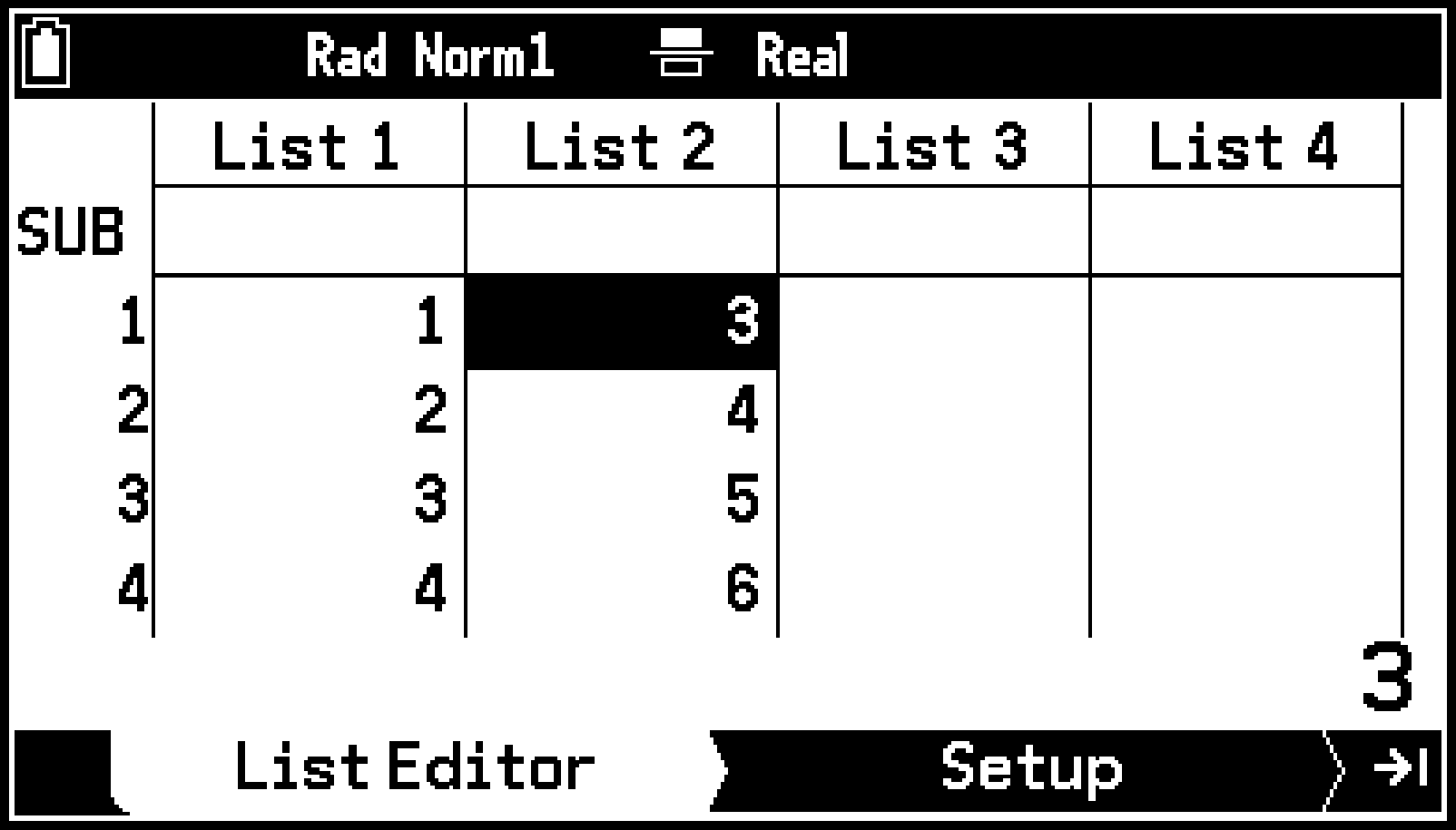
Input “List 1+2”.
-
Press E.
V > [List] > [List 1]+2
Note
You can also use the Calculate app to manipulate list variables. See Storing List Variables.
Using the List Editor Tab
To edit cell contents
|
To do this: |
Perform this operation: |
|---|---|
|
Replace the value of a cell |
Highlight the cell and input a new value. |
|
Edit the contents of a cell |
Highlight the cell and then select T > [Edit]. |
|
Delete the contents of a cell |
Highlight the cell and then select T > [Delete] > [One Value]. This causes all the rows below the deleted cell to be shifted up one row. |
|
Delete the contents of all cells in a particular list |
Highlight any cell in the list whose cell contents you want to delete and then select T > [Delete] > [One List]. |
|
Delete all lists on the List Editor tab |
Select T > [Delete] > [All Lists]. |
|
Insert a new cell |
Select T > [Insert]. This inserts a new cell that contains the value 0. All the cells below the inserted cell are shifted down one row. |
To give a list a sub-name
Highlight the “SUB” row of the list to which you want to give a sub-name and then input the name you want. You can input up to eight characters but only the characters that can fit within the width of the display are shown.
The “SUB” line is not displayed when the S > [Sub Name] setting is turned off.
To change the display color of a value
|
To do this: |
Perform this operation: |
|---|---|
|
Change the display color of one cell |
|
|
Change the display color of all values in a list* |
|
The color of a list’s sub-name is not affected by this operation. Also, any values you input into blank cells after performing this operation are displayed in black (default setting).
Sorting List Elements
Use the procedure below to sort the elements of a list on the List Editor tab in ascending or descending order of their values. You can specify one list to use as the base list and then simultaneously sort the elements of up to six lists accordingly.
-
Select T > [Sort/Jump] > [Sort Ascending] or [Sort Descending].
-
Specify the number of lists to be sorted and then press O.
-
Input the number of the list to use as the base list and then press O.
-
As dialogs appear, sequentially input the numbers of the other lists to be sorted.
This displays a dialog box for specifying the number of lists to sort.
This displays a dialog for specifying the base list for the sort.
If you specified one list in step 2, pressing O sorts the data in the list whose number you input here.
If you specified two or more lists in step 2, pressing O displays a dialog for specifying the second list to be sorted simultaneously.
Specifying the same list more than once results in an error. An error also occurs if you try to execute sorting and all of the lists do not have the same number of elements (lines).
List Files
Your calculator provides six list files (File 1 to File 6) that hold a total of 26 list variables (List 1 to List 26) each, which means you can store up to 156 list variables in memory. However, the calculator can handle up to 26 list variables (those in the currently open list file) at one time. To switch between list files, select S > [List File].
Importing and Exporting CSV Files
You can export the currently open list file to a CSV file. You can also import the contents of a CSV file into a list file. For details, see Using CSV Files.
Displaying Summary Statistics or Regression Model Information
You can use the procedure below to find and display various summary statistics from 1-Variable or 2-Variable statistical data. This procedure can also be used to display regression equation coefficients and coefficients of determination (referred to as “regression model information” in this manual) when regression models are applied to 2-Variable statistical data.
Operation Flow
-
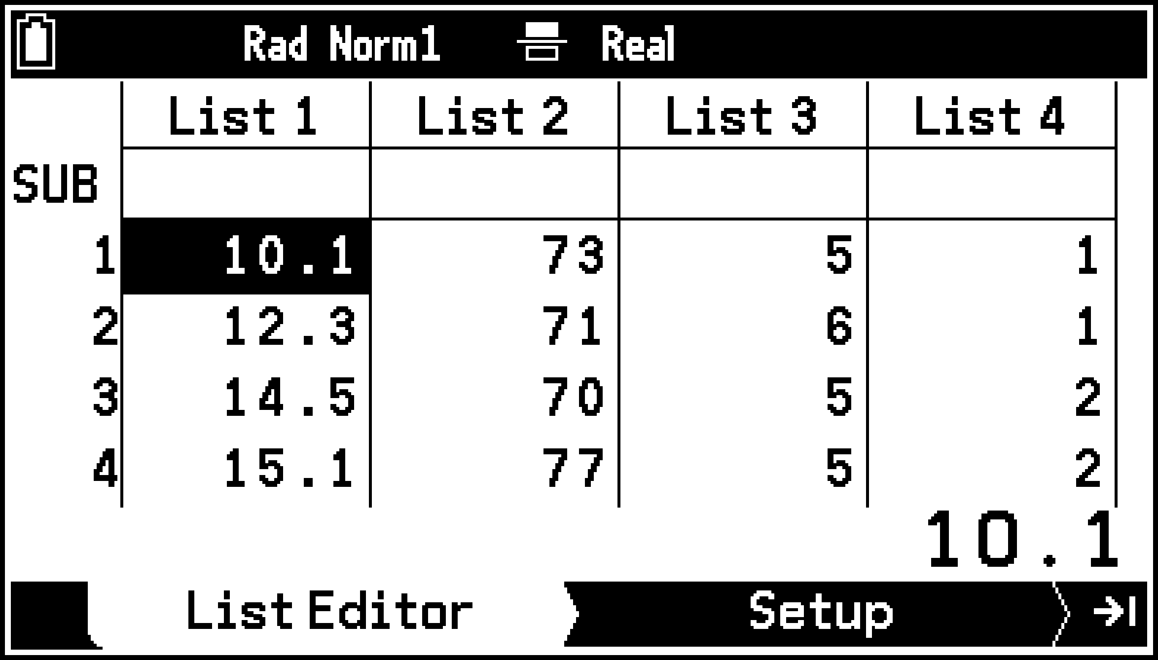
Input the statistical data to use in the calculation.
-
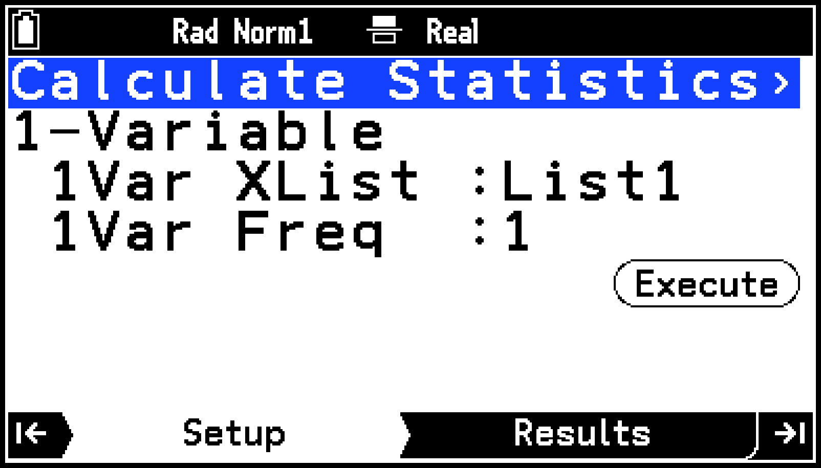
Use the procedure under Selecting What You Want to Do with the Statistics App to select [Calculate Summary Statistics].
-
Highlight line 2 on the tab and then press O.
-
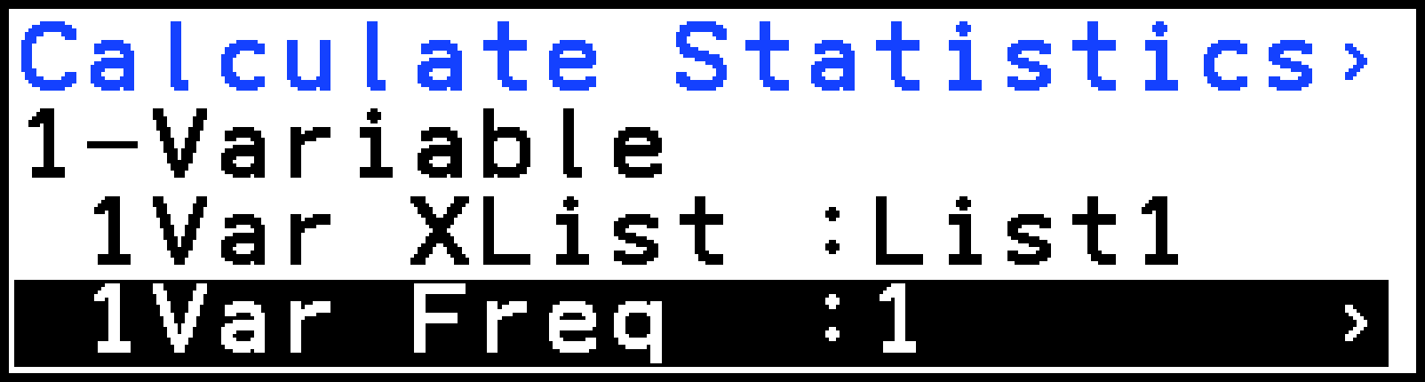
On the menu that appears, select the type of statistical calculation you want to perform.
-
If necessary, specify a list to use as statistical data.
-
Highlight [1Var XList] and then press O.
-
Use the dialog that appears to specify the number of the list variable to use as data and then press O.
-
Highlight [1Var Freq] and then press O.
-
Highlight [2Var XList] and then press O.
-
Use the dialog that appears to specify the number of the list variable to use as data for XList and then press O.
-
Highlight [2Var YList] and then press O.
-
Use the dialog that appears to specify the number of the list variable to use as data for YList and then press O.
-
Highlight [2Var Freq] and then press O.
-
Press >. Or highlight
 and then press O.
Use List Editor to input the data and then create the list variables you need. For details, see Inputting Data.
This causes the Calculate Statistics menu to appear on the Setup tab.
|
To do this: |
Select this menu item: |
|---|---|
|
Display summary statistics based on 1-Variable statistical data (X) |
1-Variable |
|
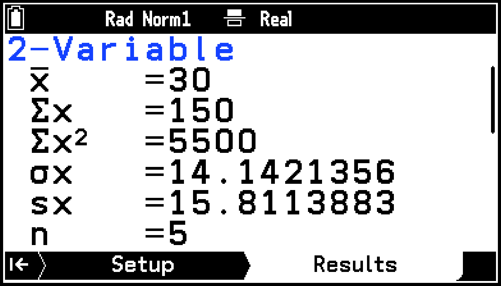
Display summary statistics based on 2-Variable statistical data (X, Y) |
2-Variable |
|
Display regression model information based on 2-Variable statistical data (X, Y) |
Linear Regression(a+b) |
|
Linear Regression(a+b) |
|
|
Med-Med Regression |
|
|
Quadratic Regression |
|
|
Cubic Regression |
|
|
Quartic Regression |
|
|
Logarithm Regression |
|
|
Exp Regression(a・e^b) |
|
|
Exp Regression(a・b^) |
|
|
Power Regression |
|
|
Sinusoidal Regression |
|
|
Logistic Regression |
For 1-Variable statistical data:
For 2-Variable statistical data:
This displays the summary statistics or regression model information you selected in step 4 on the Results tab. If a scroll bar appears along the right edge of the window, use d and u to scroll the display.
See Summary Statistics and Regression Model Information for the meanings of the values that appear on the display.
Summary Statistics
1-Variable
|
mean |
|
|
sum |
|
|
sum of squares |
|
|
population standard deviation |
|
|
sample standard deviation |
|
|
n |
number of data |
|
minX |
minimum value |
|
Q1 |
first quartile* |
|
Med |
median |
|
Q3 |
third quartile* |
|
maxX |
maximum value |
|
Mod |
mode |
|
Mod:n |
number of data mode items |
|
Mod:F |
data mode frequency |
The Q1 and Q3 calculation method is in accordance with the S > [Q1Q3 Type] setting. For details, see Q1Q3 Type (Statistics).
2-Variable
|
mean of the XList data |
|
|
sum of the XList data |
|
|
sum of squares of the XList data |
|
|
population standard deviation of the XList data |
|
|
sample standard deviation of the XList data |
|
|
n |
number of data |
|
mean of the YList data |
|
|
sum of the YList data |
|
|
sum of squares of the YList data |
|
|
population standard deviation of the YList data |
|
|
sample standard deviation of the YList data |
|
|
sum of products of the XList data and YList data |
|
|
minX |
minimum value of the XList data |
|
maxX |
maximum value of the XList data |
|
minY |
minimum value of the YList data |
|
maxY |
maximum value of the YList data |
Note
The value of each summary statistic of 1-Variable above is stored in variables included in C > [Variable Data] > [Statistics] > [X] and C > [Variable Data] > [Statistics] > [Graph] (except Mod:n and Mod:F).
The value of each summary statistic of 2-Variable above is stored in variables included in C > [Variable Data] > [Statistics] > [X] and C > [Variable Data] > [Statistics] > [Y].
Regression Model Information
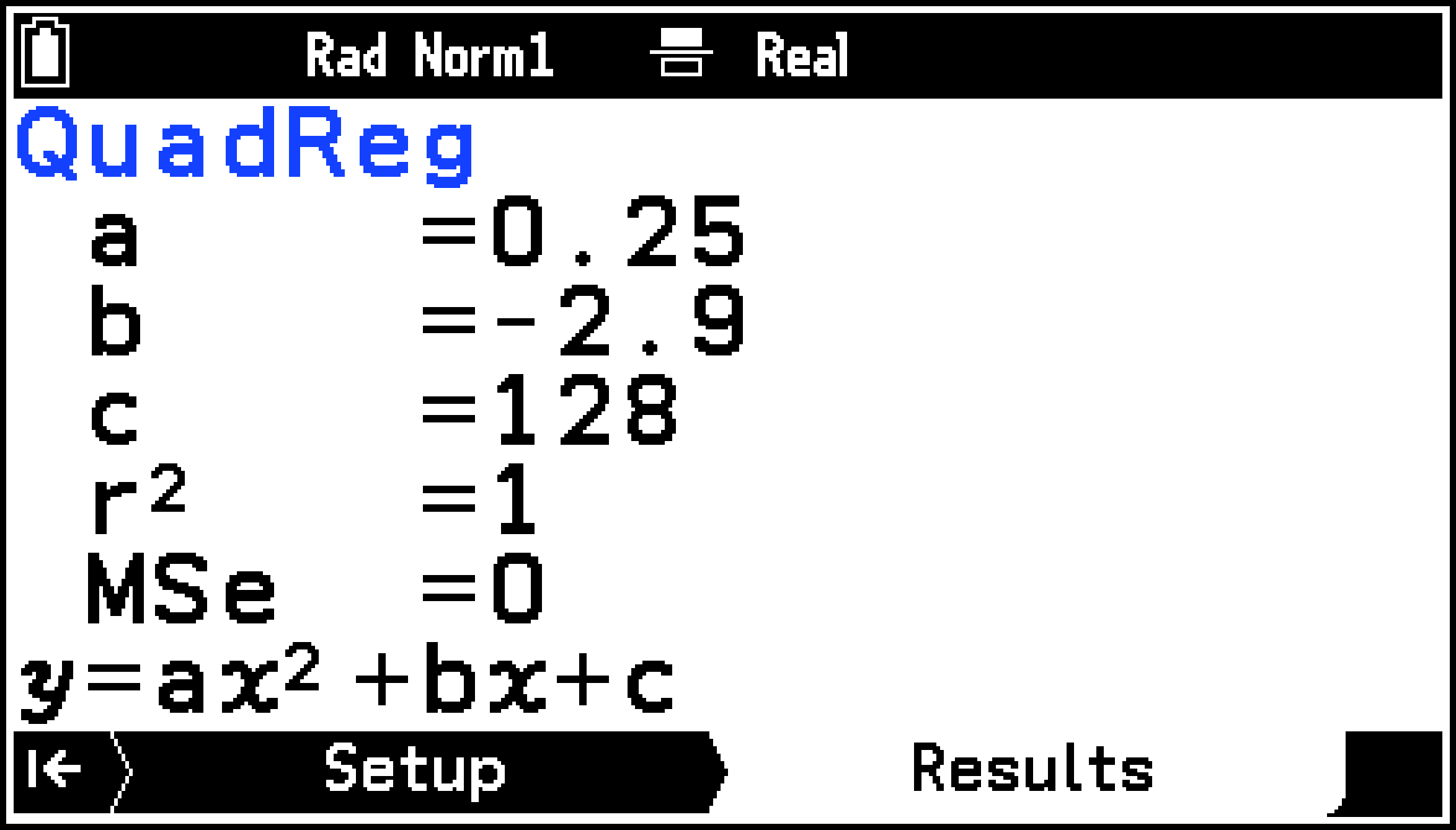
When regression model information is displayed on the Results tab, the regression model name is displayed in the first line and the regression formula is in the bottom line. The information displayed according to the regression model is shown in the table below.
|
Regression Models |
Displayed Information* |
|---|---|
|
Linear Regression(a+b) |
, , , , MSe |
|
Linear Regression(a+b) |
, , , , MSe |
|
Med-Med Regression |
, |
|
Quadratic Regression |
, , , , MSe |
|
Cubic Regression |
, , , , , MSe |
|
Quartic Regression |
, , , , , , MSe |
|
Logarithm Regression |
, , , , MSe |
|
Exp Regression(a・e^b) |
, , , , MSe |
|
Exp Regression(a・b^) |
, , , , MSe |
|
Power Regression |
, , , , MSe |
|
Sinusoidal Regression |
, , , , MSe |
|
Logistic Regression |
, , , MSe |
, , , , : regression formula coefficients, : correlation coefficient, : coefficient of determination, MSe: mean square error
Note
Each value of the above “Displayed Information” items is stored in a variable in C > [Variable Data] > [Statistics] > [Graph].
When a Med-Med Regression calculation is performed, each of the three sets of summary point coordinates (, ; , ; , ) is stored in variables in C > [Variable Data] > [Statistics] > [Point Coordinates].
What you can do while viewing regression model information
You can perform the operations shown below while regression model information is displayed on the Results tab.
|
To do this: |
Perform this operation: |
|---|---|
|
Save the calculation result regression equation to a function variable |
|
|
Find the residuals (-) of the actual data (, ) and the values (, ) calculated by the regression model and save them to a list variable |
|
Select a function number where nothing is currently stored. Overwrite saving is not available.
Input the number of an empty list. Overwrite saving is not available.
Drawing a Statistics Graph
You can use 2-Variable statistical data to draw scatter plots and various regression graphs. 1-Variable statistical data can be used to draw seven types of graphs, including histograms and box-and-whisker diagrams. After drawing a graph, you can display summary statistics and regression model information.
Drawing Scatter Plots and Regression Graphs Using the Default Settings
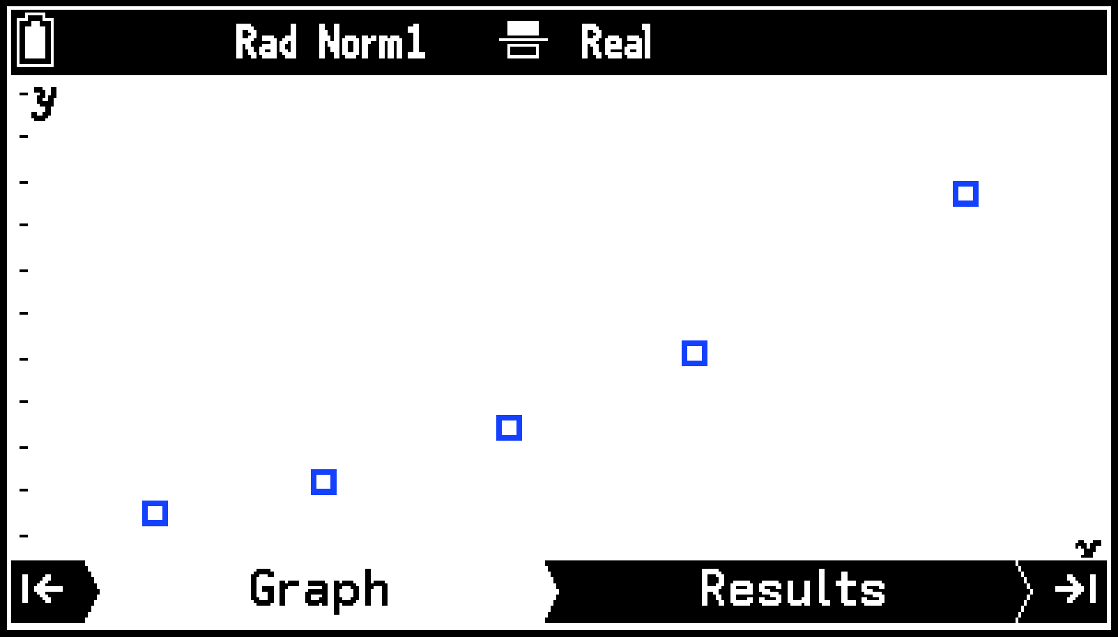
In this example, we draw a scatter plot from 2-Variable statistical data and then draw a regression graph on top of it.
-
Use List Editor to input the data below.
-
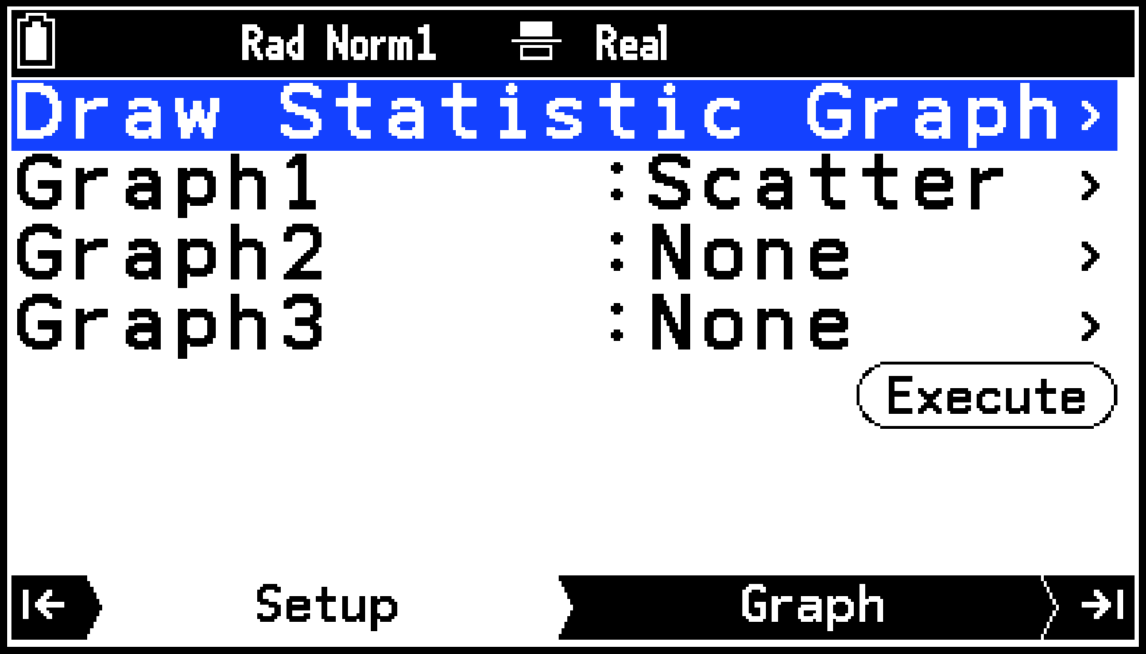
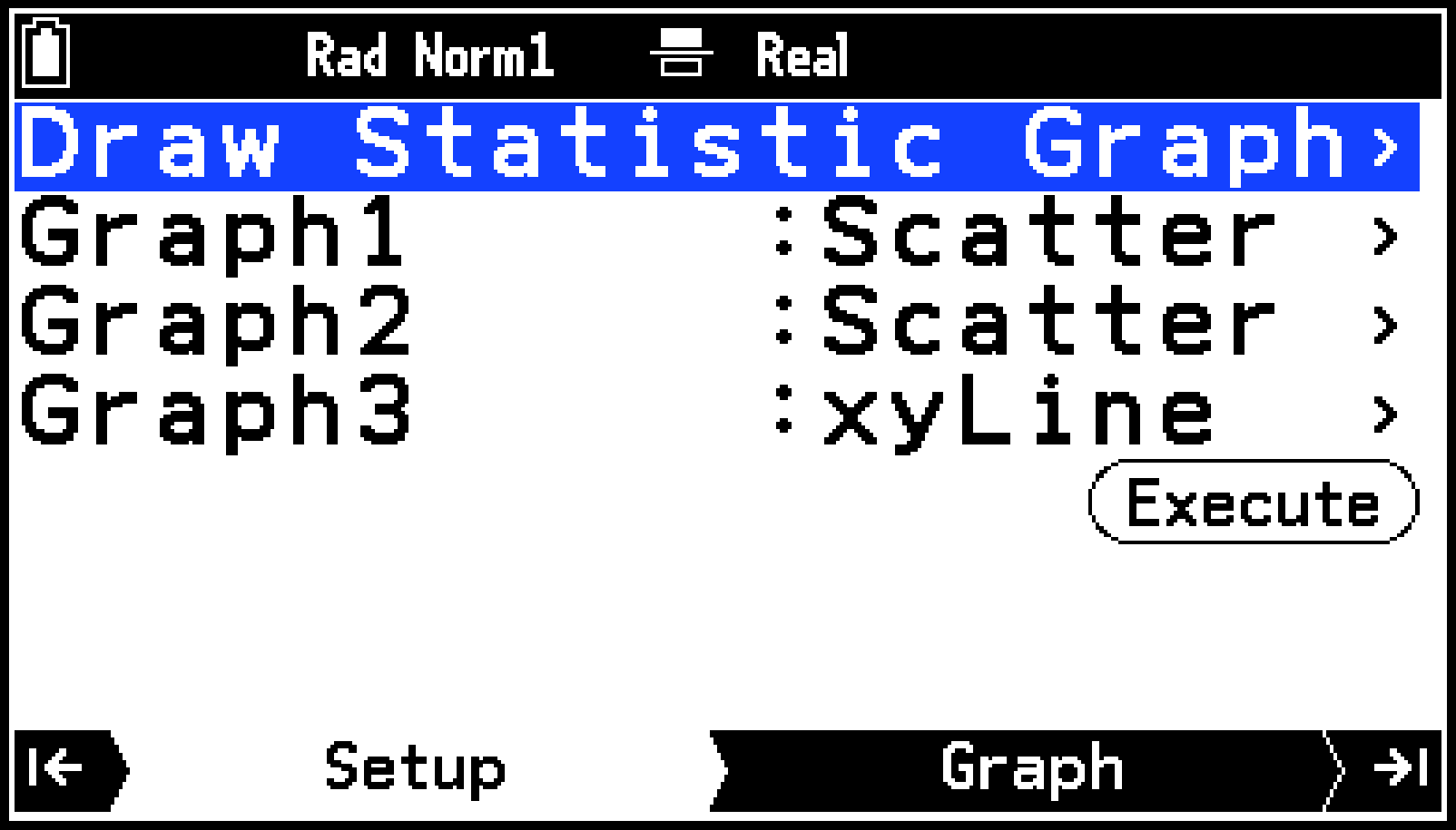
Use the procedure under Selecting What You Want to Do with the Statistics App to select [Draw Statistics Graph].
-
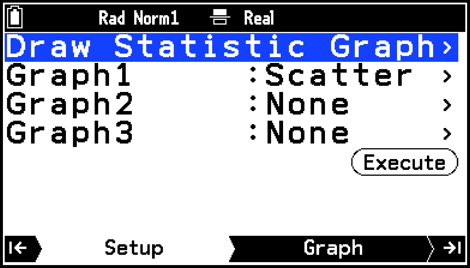
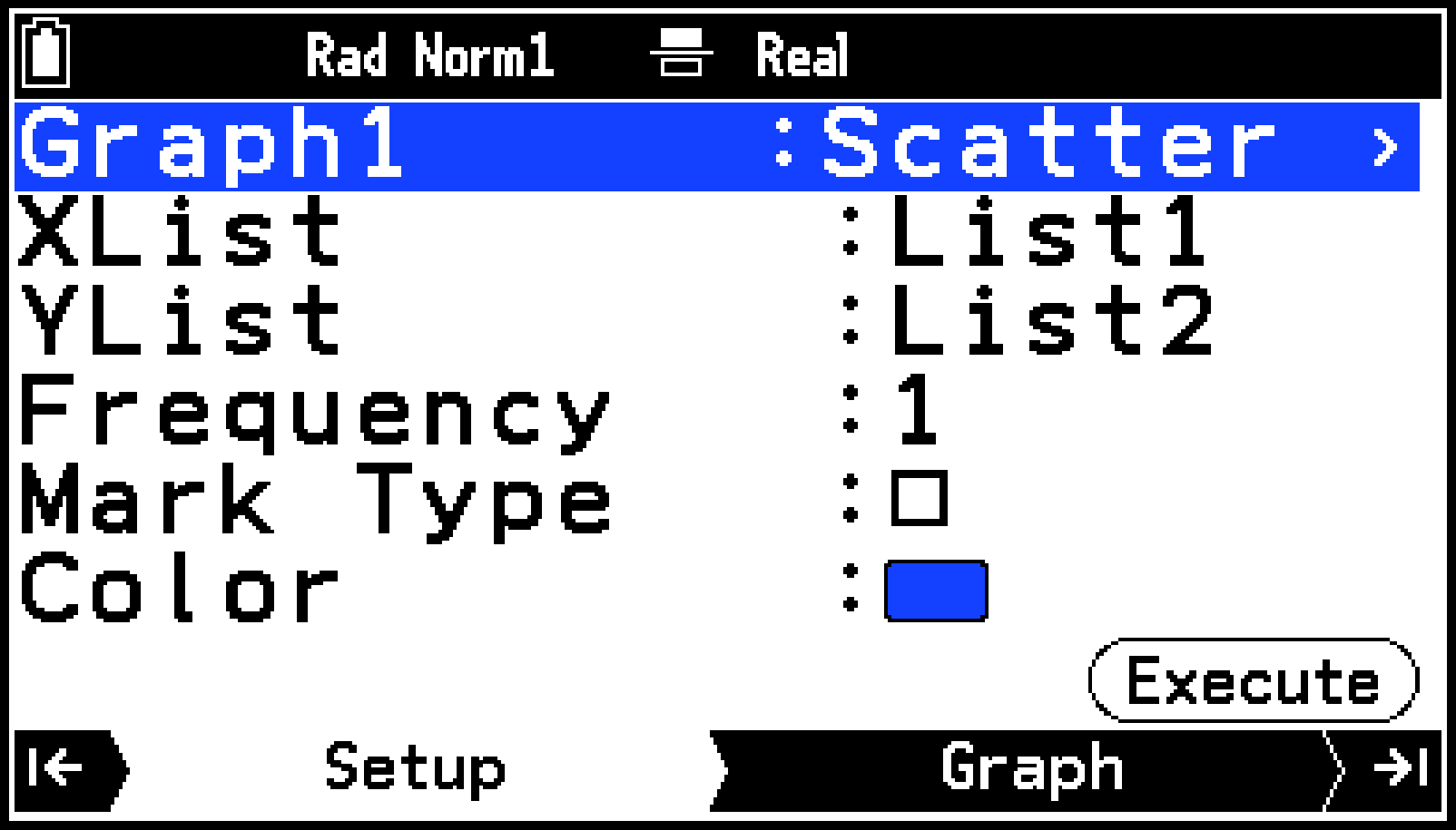
Highlight [Graph1] and then press O.
-
Press >.
-
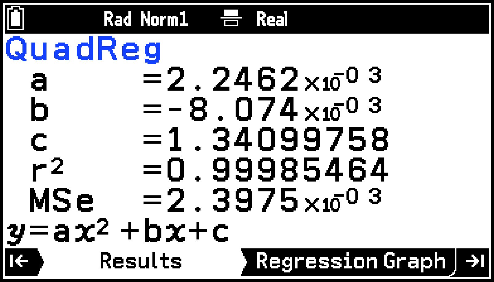
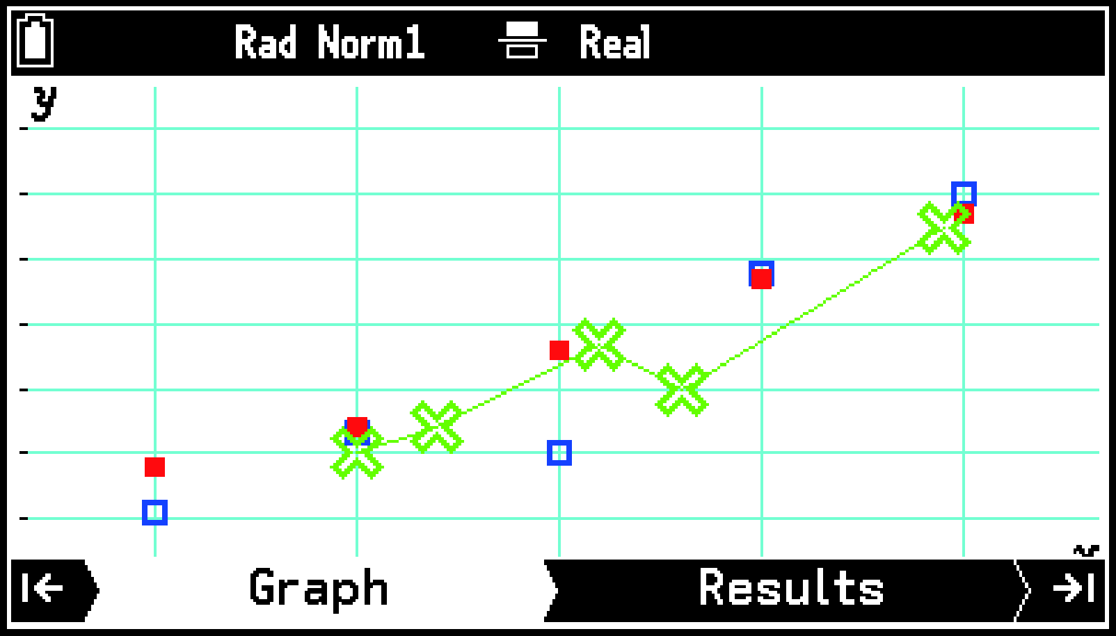
Press >. From the menu that appears, select [Quadratic Regression].
-
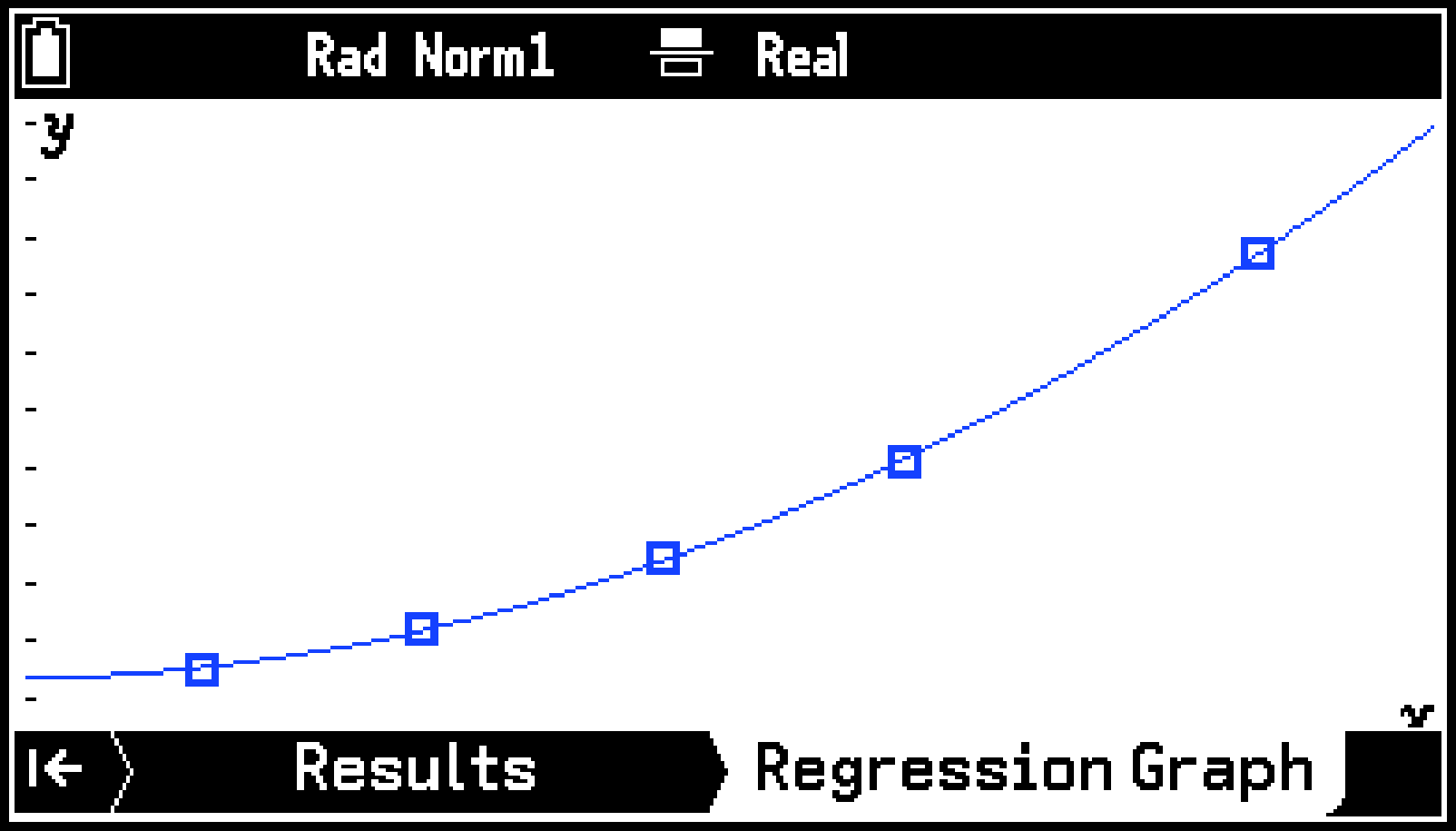
Press >.
|
List 1 |
List 2 |
|
11 |
1.5 |
|
21 |
2.2 |
|
32 |
3.4 |
|
43 |
5.1 |
|
59 |
8.7 |
For details, see Inputting Data.
This causes the Draw Statistics Graph menu to appear on the Setup tab. The default Graph1 setting is Scatter (scatter plots), and the settings of Graph2 and Graph3 are both None (Do not graph).
This causes the Setup tab display to change to the Graph1 setting menu.
By default, XList is assigned List1, YList is assigned List2, and Frequency is 1.

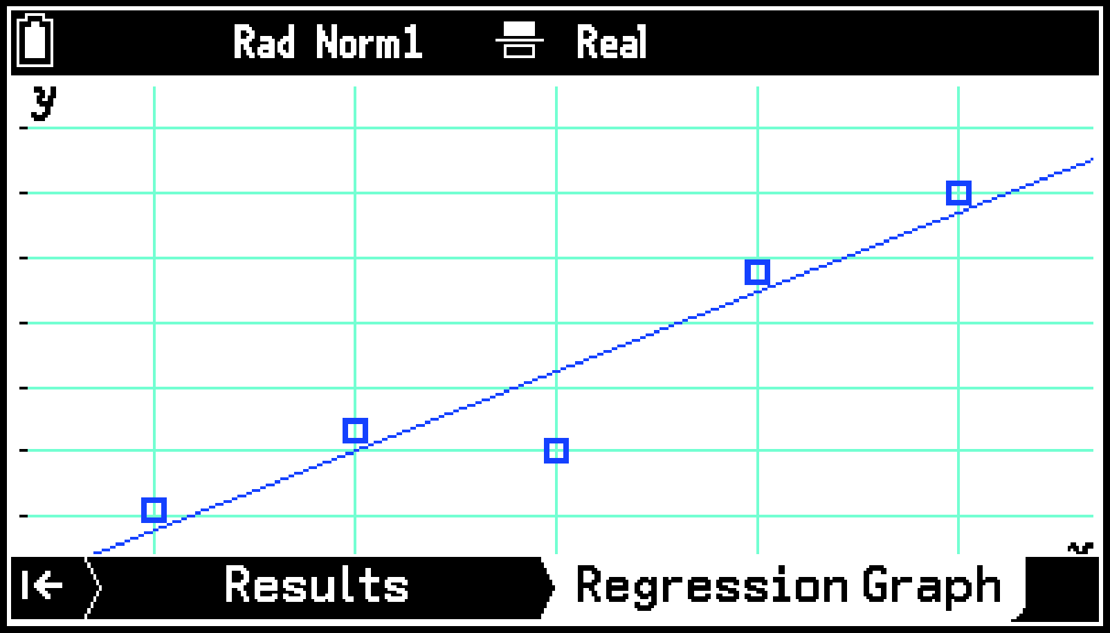
This draws a scatter plot with List1 data on the -axis and List2 data on the -axis.
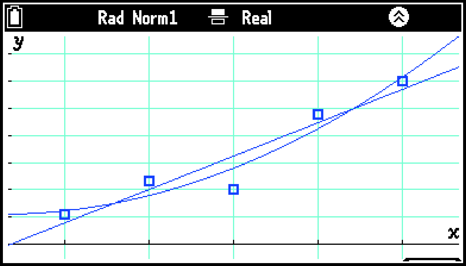
This applies a quadratic regression model to the data and displays the calculation results.
This draws a quadratic regression graph overlaid on the scatter plot.
Note
For details about Graph1 to Graph3 on the Setup tab in step 2 above, see Drawing Graphs Using Multiple Graph Setups.
For details about Graph tab operations in step 4 above and Regression Graph tab operations in step 6, see Graph Window Operations.
For the meaning of the values displayed on the Results tab in step 5 above, see Regression Model Information.
Drawing a 1-Variable Statistics Graph (Histogram, Box-and-Whisker Diagram, etc.)
You can perform the operations below based on 1-Variable statistical data you input into List Editor.
-
Draw a Box Plot, Histogram, Broken Line Graph, Pie Chart, Bar Graph, Normal Probability Plot, or Normal Density Curve.
-
Display summary statistics after drawing the graph (except for Pie Chart).
Operation Flow
-
Use List Editor to input your data.
-
Use the procedure under Selecting What You Want to Do with the Statistics App to select [Draw Statistics Graph].
-
Select the type of graph you want to draw.
-
Highlight [Graph1] and then press O.
-
Press O again.
-
Highlight the type of graph you want to draw from the menu and then press O.
-
Specify a list to use as statistical data.
-
Highlight [XList] and then press O.
-
Use the dialog that appears to specify the number of the list variable to use as data and then press O.
-
Highlight [Frequency] and then press O. (Excluding Normal Probability Plot)
-
Highlight [Data] and then press O.
-
Use the dialog that appears to specify the number of the list variable to use as data and then press O.
-
Highlight [Data1] and then press O.
-
Use the dialog that appears to specify the number of the list variable to use as data and then press O.
-
Repeat the steps (1) and (2) above for [Data2] and [Data3].
-
Specify the graph color and other settings as required.
-
To draw the graph, press >. Or highlight
and then press O. -
To view summary statistics, press >. (This operation cannot be used for a Pie Chart.)
For details, see Inputting Data.
This causes the Draw Statistics Graph menu to appear on the Setup tab.
This causes the Setup tab display to change to the Graph1 setting menu.
This displays a menu for selecting the graph type.
For a Box Plot, Histogram, Broken Line Graph, Normal Probability Plot, or Normal Density Curve:
For a Pie Chart:
When drawing a Pie Chart, you can use a maximum of 20 list variables (number of rows in a list).
For a Bar Graph:
You can specify up to three list variables as data for drawing bar graphs.
When using multiple list variables, make sure that the number of elements in all of them is the same. If all of the list variables do not have the same number of elements, an error (Dimension ERROR) results.
When using two list variables, assign them to [Data1] and [Data2]. Assigning list variables to [Data1] and [Data3] and specifying None for [Data2] results in an error (Condition ERROR).
For details, see Setting Items for Each 1-Variable Statistics Graph Type.
The graph is displayed on the Graph tab.
If the graph you selected in step 3-(2) is a Histogram or Broken Line Graph, a dialog box appears where you can specify Start (-coordinate of the graph drawing start point) and Width (graph drawing width). Input each of the values, highlight ![]() , and then press O.
, and then press O.
For information about the operations you can perform on the Graph tab, see Graph Window Operations.
This causes the summary statistics to appear on the Results tab. You can use d and u to scroll the display contents.
For the meanings of the displayed summary statistics values, see Summary Statistics.
Setting Items for Each 1-Variable Statistics Graph Type
Box Plot
Outliers:
Shows or hides outlier dots in a Box Plot.
[On]: Show
[Off]: Hide
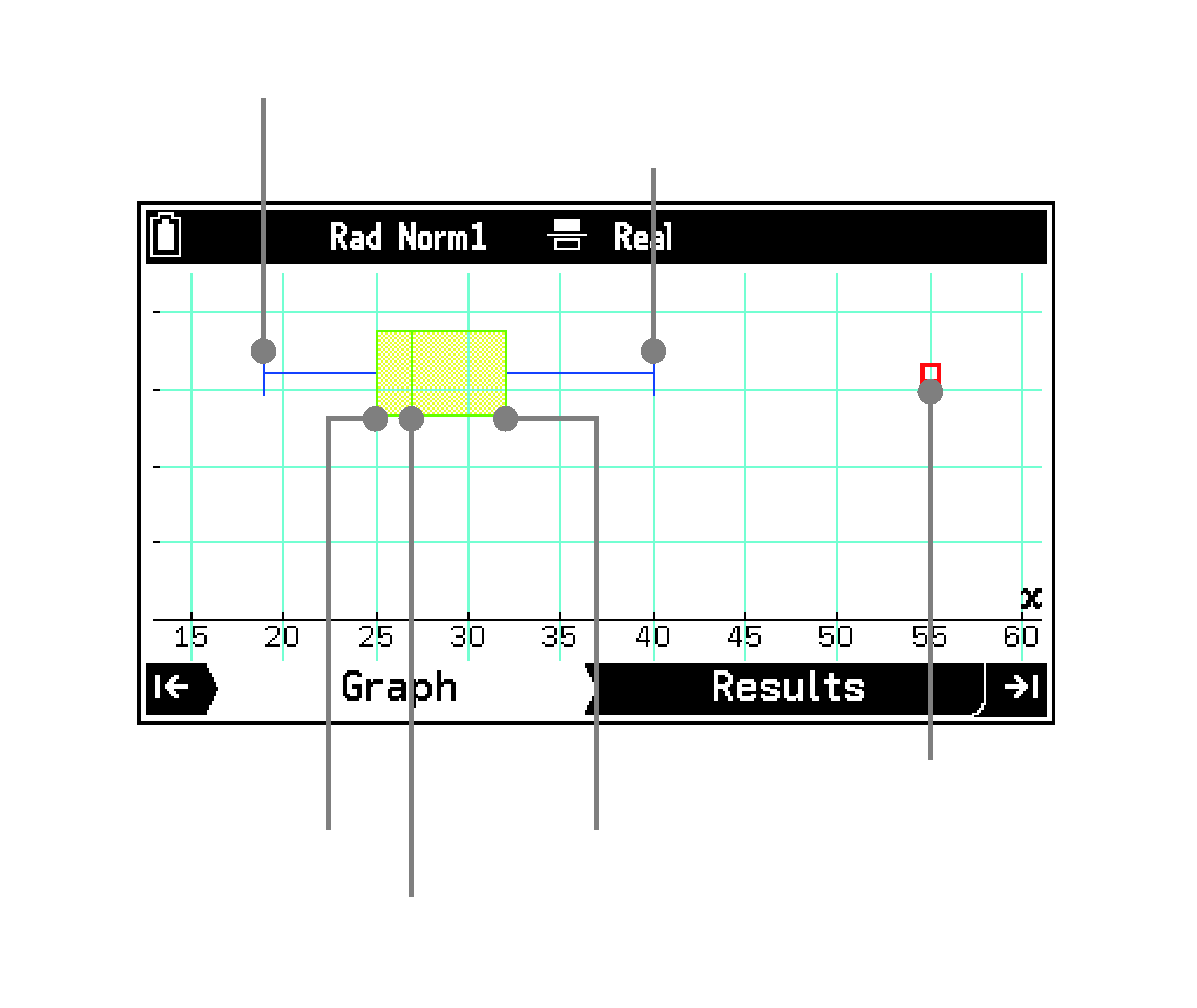
minX
Q1
Med
Q3
maxX
Outlier dot
Box:
Specifies the color of the border of the box area from Q1 to Q3, and the Med line.
Whisker:
Specifies the color of the lines extending from the ends of the box to minX and maxX.
OutlierColor:
Specifies the color of the outlier dots.
Box Inside:
Specifies the fill color of the box area from Q1 to Q3.
- Area Color:
Specifies the fill color.
Selecting [Auto] fills the area inside of the box from Q1 to Med with blue and fills the inside of the box from Med to Q3 with yellow.
- Paint Style:
Specifies the density of the fill color.
[Normal]: Normal density fill
[Lighter]: Lighter density fill
Note
Changing the S > [Q1Q3 Type] setting may alter the position of Q1 and Q3 even if Box Plot is drawn based on the same data.
Histogram
Area:
Specifies the fill color of the histogram.
- Area Color:
Specifies the fill color.
Selecting [Auto] automatically colors each data item, cycling through six colors in the following sequence: blue, red, green, magenta, cyan, yellow.
- Paint Style:
Same as Box Plot.
Border:
Specifies the histogram border color. A border is not drawn if [Clear] is selected.
Broken Line Graph
Color:
Specifies the graph draw color.
Pie Chart
Display:
Specifies the data display form.
[%]: Percentages
[Data]: Values
Pie Area:
Specifies the fill color of the pie chart.
- Area Color:
Same as Histogram.
- Paint Style:
Same as Box Plot.
Pie Border:
Specifies the border color of the pie chart. A border is not drawn if [Clear] is selected.
Bar Graph
Stick Style:
Specifies the orientation of the bars.
[Length]: Vertical
[Horizontal]: Horizontal
D1 Area, D2 Area, D3 Area:
Specifies the fill color of each bar for Data1, Data2, and Data3
- Area Color:
Same as Histogram.
- Paint Style:
Same as Box Plot.
D1 Border, D2 Border, D3 Border:
Specifies the border color of each bar for Data1, Data2, and Data3. Borders are not drawn if [Clear] is selected.
Normal Probability Plot
Mark Type:
Specifies the mark to use for the plot.
Color:
Specifies the graph draw color.
Normal Density Curve
Color:
Specifies the graph draw color.
Drawing a 2-Variable Statistics Graph (Scatter Plot or Regression Graph)
You can perform the operations below based on 2-Variable statistical data you input into List Editor.
-
Draw a Scatter Plot, xy Line Graph, or regression graph
-
After drawing a graph, display summary statistics or regression model information
-
Draw a regression graph over a graph described in (1) above*
Common practice in (1) is to draw a Scatter Plot and then draw a regression graph over it. You can also draw a regression graph over a xy Line Graph or another regression graph.
Operation Flow
-
Use List Editor to input your data.
-
Use the procedure under Selecting What You Want to Do with the Statistics App to select [Draw Statistics Graph].
-
Select the type of graph you want to draw.
-
Highlight [Graph1] and then press O.
-
Press O again.
-
Highlight the type of graph you want to draw from the menu and then press O.
-
Specify a list to use as statistical data.
-
Highlight [XList] and then press O.
-
Use the dialog that appears to specify the number of the list variable to use as data for XList and then press O.
-
Highlight [YList] and then press O.
-
Use the dialog that appears to specify the number of the list variable to use as data for YList and then press O.
-
Highlight [Frequency] and then press O. (This operation does not work with a Sinusoidal Regression Graph or Logistic Regression Graph.)
-
Specify the graph color and other settings as required.
-
To draw the graph, press >. Or highlight
and then press O. -
Display summary statistics or regression model information.
-
Press >.
-
Perform the operations described in the table below.
-
Press O.
-
Press > to go to the Regression Graph tab and draw a regression graph.
-
Add regression graphs as needed.
-
Select T > [Draw Regression Graph].
-
From the menu that appears, select the regression model you want and then press O.
For details, see Inputting Data.
This causes the Draw Statistics Graph menu to appear on the Setup tab.
This causes the Setup tab display to change to the Graph1 setting menu.
This displays a menu for selecting the graph type.
The menu includes both 1-Variable and 2-Variable graphs. Choose Scatter Plot, xy Line Graph, or regression graph.
Mark Type: If you selected Scatter Plot or xy Line Graph as the graph type, specify the mark to use for the plot.
Color: Specifies the graph draw color.
The graph is displayed on the Graph tab.
For information about the operations you can perform on the Graph tab, see Graph Window Operations.
|
To display this information: |
Select this menu item: |
|---|---|
|
Summary statistics |
2-Variable |
|
Regression model information |
Linear Regression(a+b) |
|
Linear Regression(a+b) |
|
|
Med-Med Regression |
|
|
Quadratic Regression |
|
|
Cubic Regression |
|
|
Quartic Regression |
|
|
Logarithm Regression |
|
|
Exp Regression(a・e^b) |
|
|
Exp Regression(a・b^) |
|
|
Power Regression |
|
|
Sinusoidal Regression |
|
|
Logistic Regression |
This displays the details of the menu item you selected in step (2) above on the Results tab.
See Summary Statistics and Regression Model Information for the meanings of the displayed values.
Choosing one of the regression models in step 7 draws a regression graph over the graph drawn in step 6.
Choosing 2-Variable displays only the graph drawn in step 6.
You can add multiple regression graphs on the Regression Graph tab. To do this, perform the steps below.
This adds the graph of the regression model you selected.
You can repeat steps (1) and (2) above to add more regression graphs.
For operations that are available on the Regression Graph tab, see Graph Window Operations.
Graph Window Operations
This section describes operations available with the Statistics app’s graph window (Graph tab or Regression Graph tab).
Pie Chart Only Operations
The operations below are available while a Pie Chart is displayed.
|
To do this: |
Perform this operation: |
|---|---|
|
Toggle displayed values between data values and percentages |
Select T > [%/Data]. |
|
Save displayed Pie Chart percentage values to a list variable |
|
To show or hide tabs
To move the graph window up, down, left, or right
Use the cursor keys.
To zoom the graph window in or out
Press + to zoom in or - to zoom out.
Using Trace (Trace)
Trace displays a cross pointer (![]() ) on a graph, which you can use to read the coordinate values at a specific location. To enable trace, select T > [Trace]. The operations that can be performed while the trace function is enabled are described in the table below.
) on a graph, which you can use to read the coordinate values at a specific location. To enable trace, select T > [Trace]. The operations that can be performed while the trace function is enabled are described in the table below.
|
To do this: |
Perform this operation: |
|---|---|
|
Move the pointer along the graph |
Press l or r. |
|
When there are multiple graphs, move the pointer between them |
Press d or u. |
|
Exit trace |
Press b. |
Using Zoom (Zoom)
The menu items of T > [Zoom] can be used to change the display range of the graph window. For details, see Changing the Graph Window Zoom Setting (Zoom). The Statistics app’s zoom does not support [Zoom Auto].
To specify the display range of the graph window (View Window)
See Statistics Graph View Window Settings.
Using Sketch (Sketch)
You can use sketch to draw dots, lines, and text within the graphing area. For details, see Using Sketch (Sketch). The menu items below are available with the Statistics app.
[Clear Screen], [Plot], [Line], [Circle], [Vertical Line], [Horizontal Line], [Pen], [Text]
To graph a function input with the Graph&Table app (Draw Function)
While a 2-Variable graph is displayed, you can use the operation below to overlay graphs of functions.
-
Select T > [Draw Function].
-
On the menu that appears, highlight the function you want to graph and then press O.
To find the -values for -values on a regression graph (Graph Solve)
While a regression graph is displayed, you can use the operation below to find the -value for any -value on the graph.
-
Select T > [Graph Solve] > [y-Cal].
-
Use the dialog that appears to input the -value and then press O.
-
To exit this operation, press b.
The - and -coordinate values on the regression graph are displayed at the bottom of the window.
If both the - and -coordinate values are within the window’s range, a pointer appears at the coordinates on the graph.
To redisplay the dialog and input another -value, press O.
To adjust the background image (Fade I/O)
You can use this operation to adjust the opacity of the background image. See Adjusting the Graph Window Background Image (Fade I/O).
Drawing Graphs Using Multiple Graph Setups
Graph1, Graph2, and Graph3 in the Draw Statistics Graph menu are independent areas for configuring graph settings. By default, None (Do not graph) is specified for Graph2 and Graph3, and only the Graph1 settings are used for graphing.
If you want, you can use two or three graph setups to simultaneously draw multiple graphs.
Note the points below when using multiple graph setups for graphing.
Pressing > to go from the Graph tab to the Results tab displays a menu for selecting a graph setup. Choose a graph setup from the menu and press O.
Graph setups for a 1-Variable graph in one area and a 2-Variable graph in another area cannot be used to draw simultaneous graphs.
When drawing a Pie Chart or Bar Graph, only the graph setup for the graph you are drawing should be assigned to an area. None should be specified for the other areas. In the case of a Pie Chart or Bar Graph, you can draw using only one graph setup at a time.
Performing a Hypothesis Test
Statistical hypotheses are tested in a variety of ways and results are presented numerically and graphically.
Operation Flow
-
Use List Editor to input the data and then create the list variables as required.
-
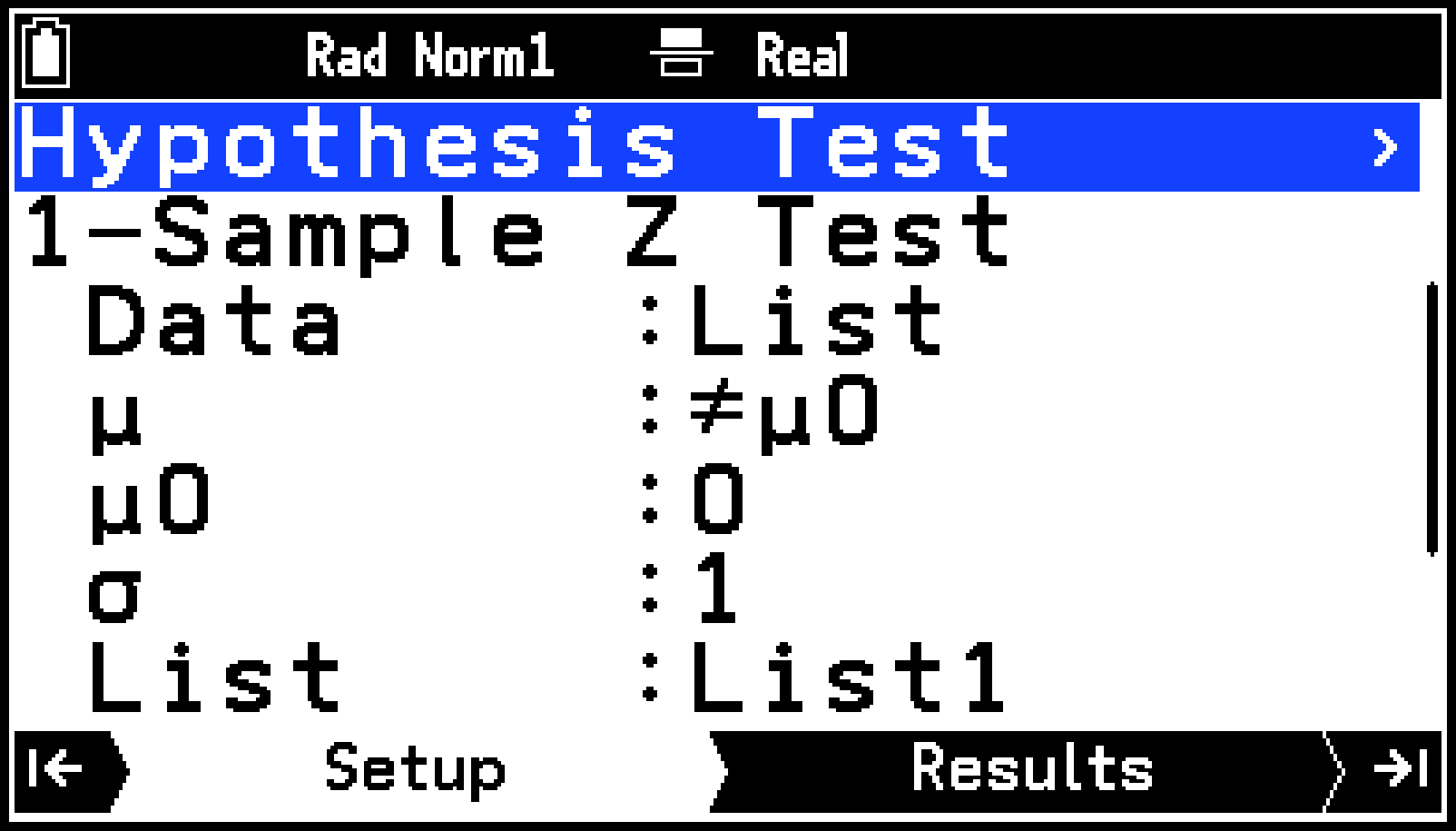
Use the procedure under Selecting What You Want to Do with the Statistics App to select [Hypothesis Test].
-
Select a test type.
-
Highlight line two of the Hypothesis Test menu and then press O.
-
From the menu that appears, select a test type.
-
Select the sample data specification method.
-
Highlight [Data] and then press O.
-
Perform the operations described in the table below.
-
Input the parameters for the alternative hypothesis.
-
Highlight [] and then press O.
-
On the menu that appears, highlight the direction of the test (≠, <, or >) and then press O.
-
Highlight [], input the numeric value of the hypothetical population mean, and then press O.
-
Input the other parameters.
-
Specify the graph color as required.*2
-
Highlight [Color] and then press O.
-
On the menu that appears, highlight the color you want and then press O.
-
Press >. Or highlight
and then press O. -
To display the graph, press >.*2
For details about the input operation, Inputting Data.
Create list variables only as needed for the test type. See Test Types and List Variables. You need to create a list variable if you want to perform a Linear Regression -Test, Goodness-of-Fit Test, or ANOVA.
This displays the Hypothesis Test menu on the Setup tab.
|
To select this: |
Select this menu item: |
Result: |
|---|---|---|
|
1-Sample Test |
[Z Test] > [1-Sample Z Test] |
To Step 4 |
|
2-Sample Test |
[Z Test] > [2-Sample Z Test] |
|
|
1-Proportion Test |
[Z Test] > [1-Proportion Z Test] |
To Step 5 |
|
2-Proportion Test |
[Z Test] > [2-Proportion Z Test] |
|
|
1-Sample Test |
[t Test] > [1-Sample t Test] |
To Step 4 |
|
2-Sample Test |
[t Test] > [2-Sample t Test] |
|
|
Linear Regression Test |
[t Test] > [Linear Regression t Test] |
To Step 5 |
|
Goodness-of-Fit Test |
[ Test] > [ Goodness-of-Fit Test] |
To Step 6 |
|
Two-Way Test |
[ Test] > [ Two-Way Test] |
|
|
2-Sample Test |
[2-Sample F Test] |
To Step 4 |
|
ANOVA |
[ANOVA] |
To Step 6 |
|
To do this: |
Perform this operation: |
|---|---|
|
Use a list variable to specify the sample data |
On the menu that appears, highlight [List] and then press O. |
|
Input the sample mean, standard deviation,*1 and number of data points |
On the menu that appears, highlight [Variable] and then press O. |
No input is required for the test.
For information about sample type-specific parameters, see Test Types and Parameters.
For example, if you chose [Z Test] > [1-Sample Z Test] in step 3, perform the steps below.
For information about sample type-specific parameters, see Test Types and Parameters.
This displays, on the Results tab, test calculation results and input values (or summary statistics calculated from the specified data).
For a description of the calculation results displayed and the operations available on the Results tab, see Using the Test Results Tab.
For operations that can be performed on the Graph tab, see Using the Test Graph Tab.
This operation is not required in the following cases.
When the test type is Linear Regression Test
When the test type is ANOVA, with [How Many] > [1] specified
Test Types and List Variables
Depending on the type of test you want to perform, input data in List Editor and create list variables as described below.
Linear Regression Test
|
Required list variable(s): |
Setup tab display: |
|---|---|
|
Three list variables for use as XList ( data), YList ( data), and Freq (frequency data)* |
 |
If you are not using frequency data, you do not need the Freq list variable.
Goodness-of-Fit Test
|
Required list variable(s): |
Setup tab display: |
|---|---|
|
Two list variables used for Observed (observed counts)* and Expected (expected frequencies) |
 |
All list elements must be positive integers.
ANOVA
You can perform either One-Way ANOVA or Two-Way ANOVA. On the Setup tab, select [How Many] > [1] for One-Way ANOVA or [2] for Two-Way ANOVA.
|
ANOVA Types: |
Required list variable(s): |
Setup tab display: |
|---|---|---|
|
One-Way ANOVA |
Two list variables used for Factor A (Factor A condition) and Dependnt (sample data) |
 |
|
Two-Way ANOVA |
Three list variables used for Factor A (Factor A condition), Factor B (Factor B condition) and Dependnt (sample data) |
 |
The list variables used in ANOVA are created as described below.
One-Way ANOVA: For example, if there are two conditions (Condition 1, Condition 2) for Factor A, each list is created as shown below.
|
Factor A |
Dependent |
|
|
|---|---|---|---|
|
1 |
113 |
 |
Condition 1 sample data |
|
1 |
116 |
||
|
2 |
133 |
|
Condition 2 sample data |
|
2 |
131 |
Two-Way ANOVA: For example, if there are two different conditions (Condition 1, Condition 2) for Factor A and Factor B, each list is created as shown below.
|
Factor A |
Factor B |
Dependent |
|
|
|---|---|---|---|---|
|
1 |
1 |
113 |
|
Factor A Condition 1 × Factor B Condition 1 sample data |
|
1 |
1 |
116 |
||
|
2 |
1 |
133 |
|
Factor A Condition 2 × Factor B Condition 1 sample data |
|
2 |
1 |
131 |
||
|
1 |
2 |
139 |
|
Factor A Condition 1 × Factor B Condition 2 sample data |
|
1 |
2 |
132 |
||
|
2 |
2 |
126 |
|
Factor A Condition 2 × Factor B Condition 2 sample data |
|
2 |
2 |
122 |
1-Sample or 2-Sample Test, 1-Sample or 2-Sample Test, 2-Sample Test
If you choose [Data] > [List] in step 4 under Operation Flow, need to create the following list variables.
|
Sample data: |
Required list variable(s): |
Setup tab display: |
|---|---|---|
|
One sample data (no frequencies) |
List variable to assign to List |
 |
|
One sample data (with frequencies) |
Two list variables to assign to List and Freq |
|
|
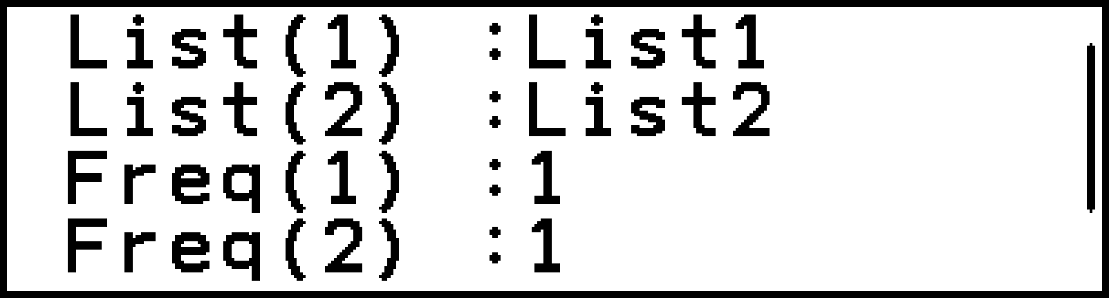
Two sample data (no frequencies) |
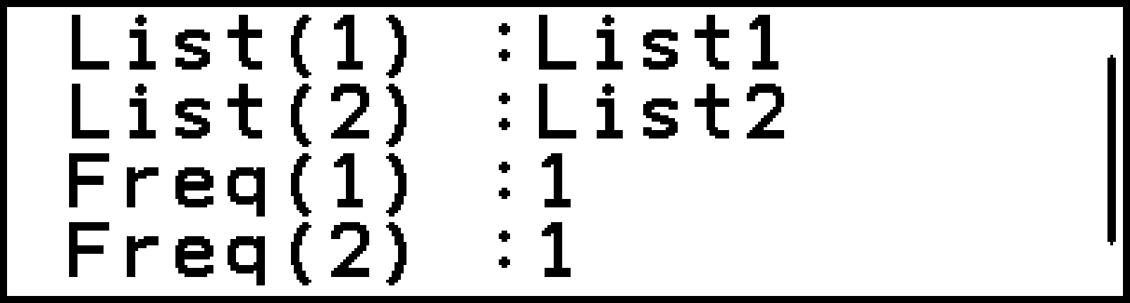
Two list variables to assign to List(1) and List(2) |
 |
|
Two sample data (with frequencies) |
Four list variables to assign to List(1), List(2), Freq(1), Freq(2) |
Test Types and Parameters
Alternative Hypothesis Parameters
|
Test Type: |
Parameter: |
|---|---|
|
1-Sample Test |
: test conditions (“≠” specifies two-tail test, “<” specifies lower one-tail test, “>” specifies upper one-tail test.) |
|
2-Sample Test |
: test conditions (“≠” specifies two-tail test, “<” specifies one-tail test where sample 1 is smaller than sample 2, “>” specifies one-tail test where sample 1 is greater than sample 2.) |
|
1-Proportion Test |
Prop: test conditions (“≠” specifies two-tail test, “<” specifies lower one-tail test, “>” specifies upper one-tail test.) |
|
2-Proportion Test |
: test conditions (“≠” specifies two-tail test, “<” specifies one-tail test where sample 1 is smaller than sample 2, “>” specifies one-tail test where sample 1 is greater than sample 2.) |
|
Linear Regression Test |
&: test conditions (“≠0” specifies two-tail test, “< 0” specifies lower one-tail test, “> 0” specifies upper one-tail test.) |
|
2-Sample Test |
: test conditions (“≠” specifies two-tail test, “<” specifies one-tail test where sample 1 is smaller than sample 2, “>” specifies one-tail test where sample 1 is greater than sample 2.) |
Other Parameters
Parameters in the table below that are marked with an asterisk (*) need to be input when you select [Data] > [Variable] in step 4 of the procedure under Operation Flow.
|
Test Type: |
Parameter: |
|---|---|
|
1-Sample Test |
: population standard deviation ( > 0) : mean of sample* : size of sample (positive integer)* |
|
2-Sample Test |
: population standard deviation of sample 1 ( > 0) : population standard deviation of sample 2 ( > 0) : mean of sample 1* : size of sample 1 (positive integer)* : mean of sample 2* : size of sample 2 (positive integer)* |
|
1-Proportion Test |
: sample value ( ≥ 0 integer) : size of sample (positive integer) |
|
2-Proportion Test |
: data value of sample 1 ( ≥ 0 integer) : size of sample 1 (positive integer) : data value of sample 2 ( ≥ 0 integer) : size of sample 2 (positive integer) |
|
1-Sample Test |
: mean of sample* : sample standard deviation ( > 0)* : size of sample (positive integer)* |
|
2-Sample Test |
: mean of sample 1* : standard deviation of sample 1 ( > 0)* : size of sample 1 (positive integer)* : mean of sample 2* : standard deviation of sample 2 ( > 0)* : size of sample 2 (positive integer)* Pooled: pooling On (in effect) or Off (not in effect) |
|
Goodness-of-Fit Test |
Observed: specify a list variable (List 1 to List 26) that contains observed counts (all list elements must be positive integers). Expected: specify a list variable (List 1 to List 26) as the storage location of expected frequency. df: degrees of freedom (positive integer) CNTRB: specify a list variable (List 1 to List 26) as the storage location of the contribution of each observed count obtained as calculation results. |
|
Two-Way Test |
Observed: Specifies a matrix variable (Mat A to Mat Z) that contains observed counts. Be sure to specify a matrix that satisfies the conditions below. An error results if you specify a matrix that does not satisfy these conditions. The matrix must have at least 2 rows and 2 columns. All elements of the matrix must be positive integers. Expected: Specifies a matrix variable (Mat A to Mat Z) that contains expected frequencies. |
|
2-Sample Test |
: standard deviation of sample 1 ( > 0)* : size of sample 1 (positive integer)* : standard deviation of sample 2 ( > 0)* : size of sample 2 (positive integer)* |
|
ANOVA |
How Many: 1: One-Way ANOVA 2: Two-Way ANOVA |
Using the Test Results Tab
Information on the Results Tab
When a test other than ANOVA is performed
Test calculation results and summary statistics of the sample data are displayed on the Results tab. The meanings of the items that appear on the display are provided below.
Test calculation results
|
: |
-value |
|
: |
score ( Test) |
|
: |
value ( Test) |
|
: |
value ( Test) |
|
: |
value ( Test) |
|
: |
estimated sample proportion (1-Proportion/2-Proportion Test) |
|
: |
estimated proportion of sample 1 (2-Proportion Test) |
|
: |
estimated proportion of sample 2 (2-Proportion Test) |
|
df: |
degrees of freedom (2-Sample Test, Linear Regression Test, Test) |
|
: |
constant term (Linear Regression Test) |
|
: |
coefficient (Linear Regression Test) |
Summary statistics of sample data
|
: |
mean of sample |
|
: |
mean of sample 1 |
|
: |
mean of sample 2 |
|
: |
sample standard deviation |
|
: |
standard deviation of sample 1 |
|
: |
standard deviation of sample 2 |
|
: |
pooled sample standard deviation |
|
: |
size of sample |
|
: |
size of sample 1 |
|
: |
size of sample 2 |
|
: |
standard error |
|
: |
correlation coefficient |
|
: |
coefficient of determination |
When ANOVA is performed
Calculation results are displayed using the same table form as that used in textbooks.
One-Way ANOVA
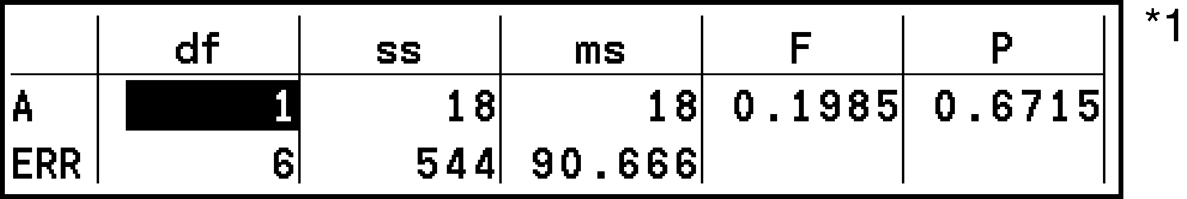
Line 1: A values
Line 2: ERR values
Two-Way ANOVA
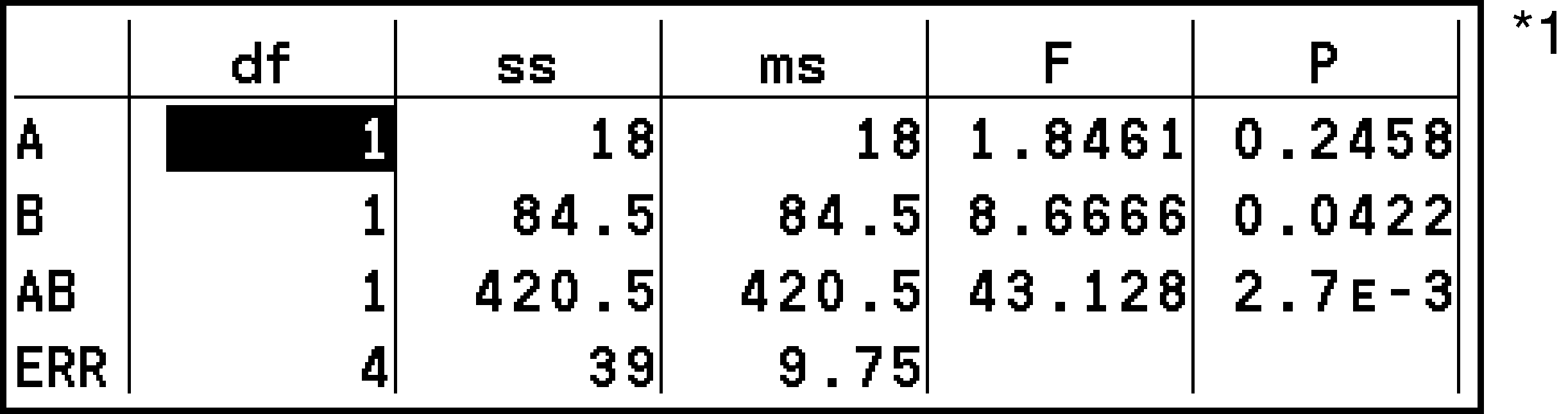
Line 1: A values
Line 2: B values
Line 3: AB values*2
Line 4: ERR values
The tables shown here would be displayed by the calculator across two screens, so you would need to scroll left and right to view all of the table contents.
Line 3 does not appear when there is only one observation in each cell.
Column 1: df ... degrees of freedom
Column 2: ss ... sum of squares
Column 3: ms ... mean squares
Column 4: F ... value
Column 5: P ... -value
Note
Values displayed on the Results tab are stored in variables in C > [Variable Data] > [Statistics] > [Result] > [Test] and C > [Variable Data] > [Statistics] > [Input]. However, variables and are in C > [Variable Data] > [Statistics] > [Graph].
What you can do while displaying calculation results
You can use the operation below to save all numeric values currently displayed on the Results tab*1 to a list variable.
-
Select T > [Save Result in List].
-
Use the dialog box that appears to input the number of the list you want to use as a save destination*2*3 and then press O.
Includes the currently displayed calculation results and input values. However, alternative hypothesis parameters are not saved.
Input the number of an empty list. Overwrite saving is not available.
With ANOVA, each of the five calculation result columns is saved to five list variables, starting from the list number you input. You can specify a list number within the range from 1 to 22.
Note
You can perform the operations described below while the calculation results of Linear Regression Test are displayed.
Save the calculation result regression equation to a function variable.
Find the residuals between the actual data and the values calculated by the regression model and save them to list variables.
See What you can do while viewing regression model information.
Using the Test Graph Tab
When you perform a test other than Two-Way ANOVA
You can perform the operations below after performing one of the following tests: 1-Sample Test, 2-Sample Test, 1-Proportion Test, 2-Proportion Test, 1-Sample Test, 2-Sample Test, Goodness-of-Fit Test, Two-Way Test, 2-Sample Test.
|
To do this: |
Select this menu item: |
|---|---|
|
Display the -value |
T > [Calculate P Value] |
|
Test: Display the -value and display a cross pointer at the corresponding point on the graph |
T > [Calculate Z Value]*1*2 |
|
1-Sample/2-Sample Test: Display the -value(s) and display a cross pointer at the corresponding point on the graph |
T > [Calculate T Value]*1*2 |
|
Test: Display the -value(s) and display a cross pointer at the corresponding point on the graph |
T > [Calculate CHI Value]*1*2 |
|
2-Sample Test: Display the -value and display a cross pointer at the corresponding point on the graph |
T > [Calculate F Value]*1*2 |
For a two-tailed test, the cross pointer moves between the two values each time l or r is pressed.
A relevant point outside of the display range is not displayed.
Note
Calculation results displayed by the above operations are stored in the alpha variables described below.
|
Test |
- and -values are stored in variables Z and P respectively. |
|
Test |
- and -values are stored in variables T and P respectively. |
|
Test |
- and -values are stored in variables C and P respectively. |
|
Test |
- and -values are stored in variables F and P respectively. |
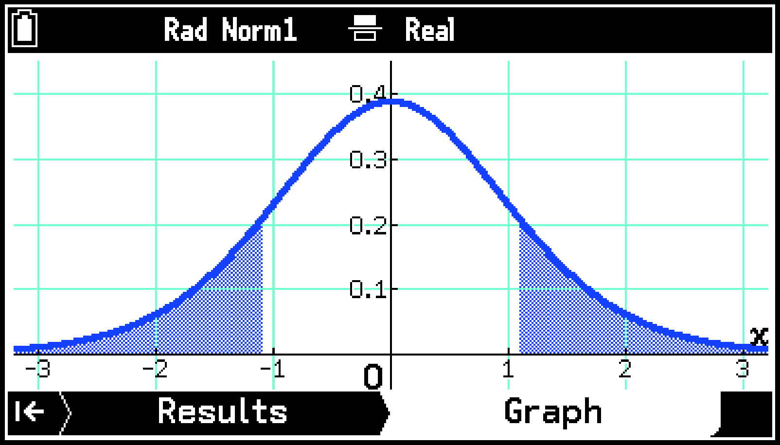
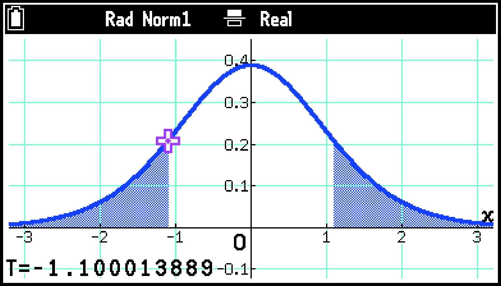
The displays below show an example of what would happen if you perform a one-sample -test with ≠ (two-tailed test) and then draw a graph. The display on the right is an example when you select T > [Calculate T Value].
When Two-Way ANOVA is performed
With Two-Way ANOVA, you can draw Interaction Plot graphs. The number of graphs depends on Factor B, while the number of -axis data depends on Factor A. The -axis is the mean value of each category.
Selecting T > [Trace] displays a cross pointer on the graph (Trace). Pressing l or r moves the pointer on the graph in the corresponding direction. When there are multiple graphs, you can use d and u to move between graphs.

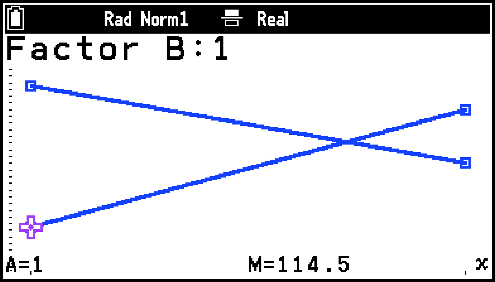
Using the Trace function automatically stores the last condition number of factor A to variable A and the mean value of the last category to variable M, respectively.
Find a Confidence Interval
You can use the procedure below to find the upper and lower limits of the confidence interval from given sample data and confidence level.
Operation Flow
-
Use List Editor to input the data and then create the list variables as required.
-
Use the procedure under Selecting What You Want to Do with the Statistics App to select [Confidence Interval].
-
Select the confidence interval type.
-
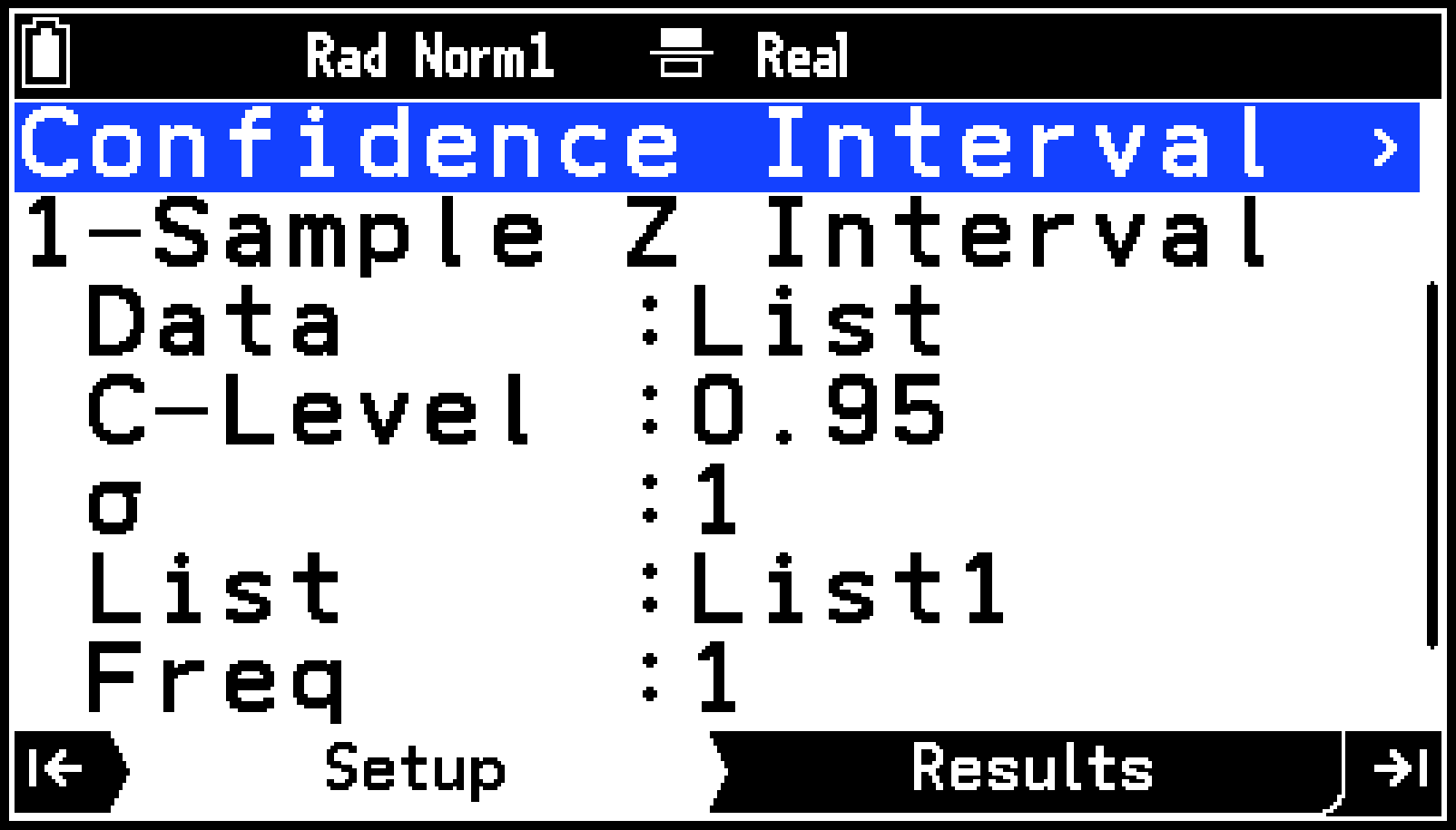
Highlight line 2 of the Confidence Interval menu and then press O.
-
From the menu that appears, select a confidence interval type.
-
Select the sample data specification method.
-
Highlight [Data] and then press O.
-
Perform the operations described in the table below.
-
Input values for the parameters.
-
Highlight [C-Level] and then use the number keys to input the confidence level.
-
Press O.
-
Input the other parameters.
-
Press >. Or highlight
and then press O.
For details about the input operation, Inputting Data.
See Confidence Interval Types and List Variables for the list variables that need to be created.
This displays the Confidence Interval menu on the Setup tab.
|
To select this: |
Select this menu item: |
Result: |
|---|---|---|
|
1-Sample Interval |
[Z Confidence Interval] > [1-Sample Z Interval] |
To Step 4 |
|
2-Sample Interval |
[Z Confidence Interval] > [2-Sample Z Interval] |
|
|
1-Proportion Interval |
[Z Confidence Interval] > [1-Proportion Z Interval] |
To Step 5 |
|
2-Proportion Interval |
[Z Confidence Interval] > [2-Proportion Z Interval] |
|
|
1-Sample Interval |
[t Confidence Interval] > [1-Sample t Interval] |
To Step 4 |
|
2-Sample Interval |
[t Confidence Interval] > [2-Sample t Interval] |
|
To do this: |
Perform this operation: |
|---|---|
|
Use a list variable to specify the sample data |
On the menu that appears, highlight [List] and then press O. |
|
Input the sample mean, standard deviation, and number of data points |
On the menu that appears, highlight [Variable] and then press O. |
Input a value between 0 and 1. Commonly used confidence levels are 0.95 (95%) and 0.99 (99%).
This displays confidence interval calculation results and summary statistics of the sample data on the Results tab. The meanings of the items that appear on the display are provided below.
Confidence interval calculation results
|
Lower: |
confidence interval lower limit |
|
Upper: |
confidence interval upper limit |
|
df: |
degrees of freedom |
|
: |
estimated sample proportion |
|
: |
estimated proportion of sample 1 |
|
: |
estimated proportion of sample 2 |
Summary statistics of sample data
|
: |
mean of sample |
|
: |
mean of sample 1 |
|
: |
mean of sample 2 |
|
: |
sample standard deviation |
|
: |
standard deviation of sample 1 |
|
: |
standard deviation of sample 2 |
|
: |
pooled sample standard deviation |
|
: |
size of sample |
|
: |
size of sample 1 |
|
: |
size of sample 2 |
Note
You can use the operation below to save values currently displayed on the Results tab to a list.
-
Select T > [Save Result in List].
-
Use the dialog that appears to input a list number* and then press O.
Input the number of an empty list. Overwrite saving is not available.
The values displayed on the Results tab are stored in the variables in the menu items shown below.
Confidence interval calculation results: C > [Variable Data] > [Statistics] > [Result] > [Confidence Interval]
Summary statistics of the sample data: C > [Variable Data] > [Statistics] > [Input]
Confidence Interval Types and List Variables
To find confidence intervals using a list of sample data, create the following list variables according to the confidence interval type.
|
Sample data: |
Required list variable(s): |
Setup tab display: |
|---|---|---|
|
One sample data (no frequencies) |
List variable to assign to List |
 |
|
One sample data (with frequencies) |
Two list variables to assign to List and Freq |
|
|
Two sample data (no frequencies) |
Two list variables to assign to List(1) and List(2) |
 |
|
Two sample data (with frequencies) |
Four list variables to assign to List(1), List(2), Freq(1), Freq(2) |
Confidence Interval Types and Parameters
Parameters in the table below that are marked with an asterisk (*) need to be input when you select [Data] > [Variable] in step 4 of the procedure under Operation Flow.
|
Confidence interval type: |
Parameter: |
|---|---|
|
1-Sample Interval |
: population standard deviation ( > 0) : mean of sample* : size of sample (positive integer)* |
|
2-Sample Interval |
: population standard deviation of sample 1 ( > 0) : population standard deviation of sample 2 ( > 0) : mean of sample 1* : size of sample 1 (positive integer)* : mean of sample 2* : size of sample 2 (positive integer)* |
|
1-Proportion Interval |
: sample value ( ≥ 0 integer) : size of sample (positive integer) |
|
2-Proportion Interval |
: data value of sample 1 ( ≥ 0 integer) : size of sample 1 (positive integer) : data value of sample 2 ( ≥ 0 integer) : size of sample 2 (positive integer) |
|
1-Sample Interval |
: mean of sample* : sample standard deviation ( > 0)* : size of sample (positive integer)* |
|
2-Sample Interval |
: mean of sample 1* : standard deviation of sample 1 ( > 0)* : size of sample 1 (positive integer)* : mean of sample 2* : standard deviation of sample 2 ( > 0)* : size of sample 2 (positive integer)* Pooled: pooling On (in effect) or Off (not in effect) |
Statistics Graph View Window Settings
The settings of the statistics graph View Window are automatically configured according to the graph being drawn. This is because the calculator selects S > [View Window] > [Auto] by default.
If you switch to S > [View Window] > [Manual], changes to View Window settings configured with the menu that appears when you select T > [View Window] in the graph window are applied to the display range of the graph window.
For details about View Window settings, see Specifying the Display Range of the Graph Window (View Window).
Note
Note that View Window parameters are set automatically for the graph types below, regardless of whether or not S > [View Window] is set to [Manual].
Pie, 1-Sample Test, 2-Sample Test, 1-Proportion Test, 2-Proportion Test, 1-Sample Test, 2-Sample Test, Goodness-of-Fit Test, Two-Way Test, 2-Sample Test (-axis only disregarded).