> Other Information > Catalog Menu Details

Catalog Menu Details

The Catalog menu, which appears when you press C, is a comprehensive list of all functions, commands, app variables,^* and symbols available on the calculator. You can select the item you want on the calculator and enter it into a calculation or expression.

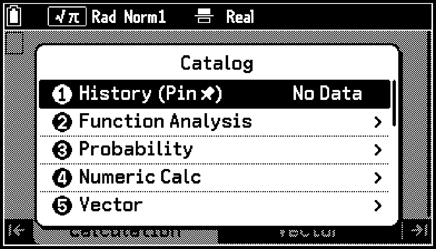
The list produced by C > [All] contains all items supported by your calculator. While the alphabetical list is displayed, you can press a key from X^A to 0^Z to display a list of items beginning with the letter you pressed.

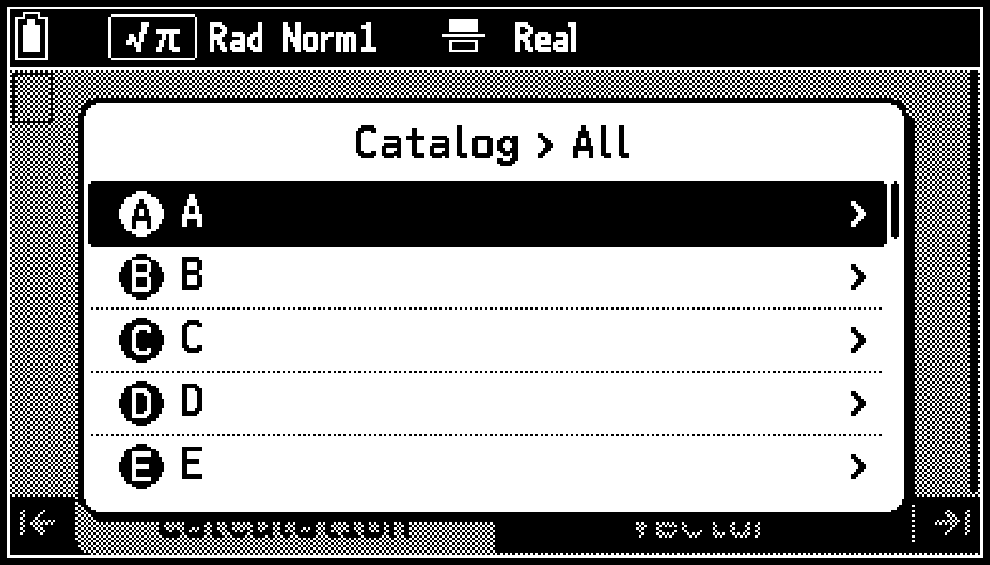
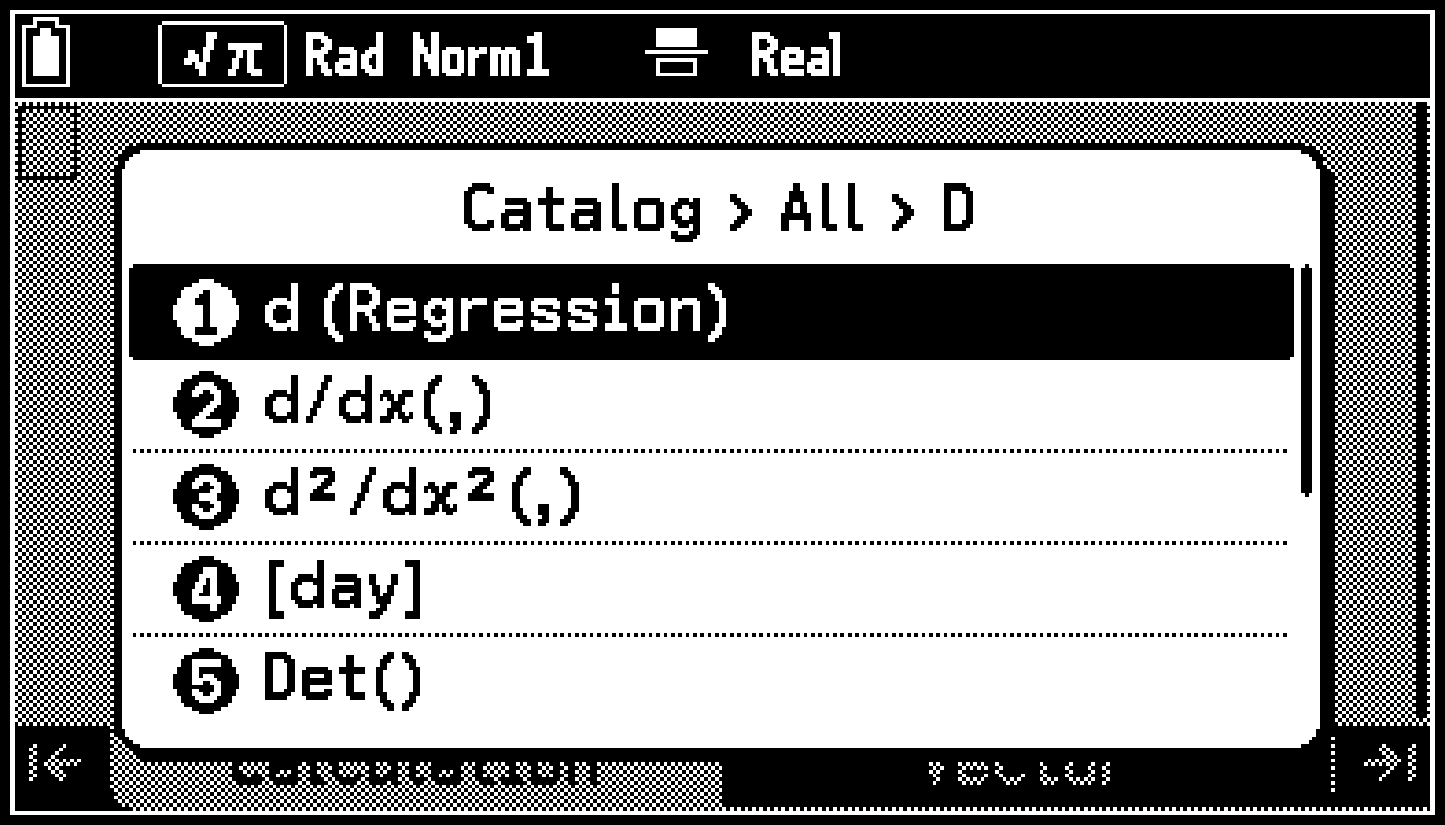
Functions and symbols that are not included in a group from [A] to [Z] can be accessed with C > [All] > [Symbol].

Items included in C > [Variable Data] (input/output variables used in an app)

Note

Pressing C while using the Python app or the Base-N app displays a Catalog menu specific to each app. For details, see the chapters explaining each app.

The Catalog menu displays the names of functions and commands in the menus by category (such as Integration‎ (∫)‎, etc.). On the C > [All] and Input History menus, the functions and commands are displayed in line input syntax (such as ∫(,,), etc.).

Using Input History

Up to 10 of the latest functions and commands^* recently entered from the Catalog menu are maintained as input history. To view the input history, select C > [History (Pin ‎ Pin )‎].

Including pinned input history.

Pinning Input History

While viewing input history, select the item you wish to pin and then press T. This causes a pin to appear to the left of the item.

The next time you open the input history, the pinned item will be at the top of the list.

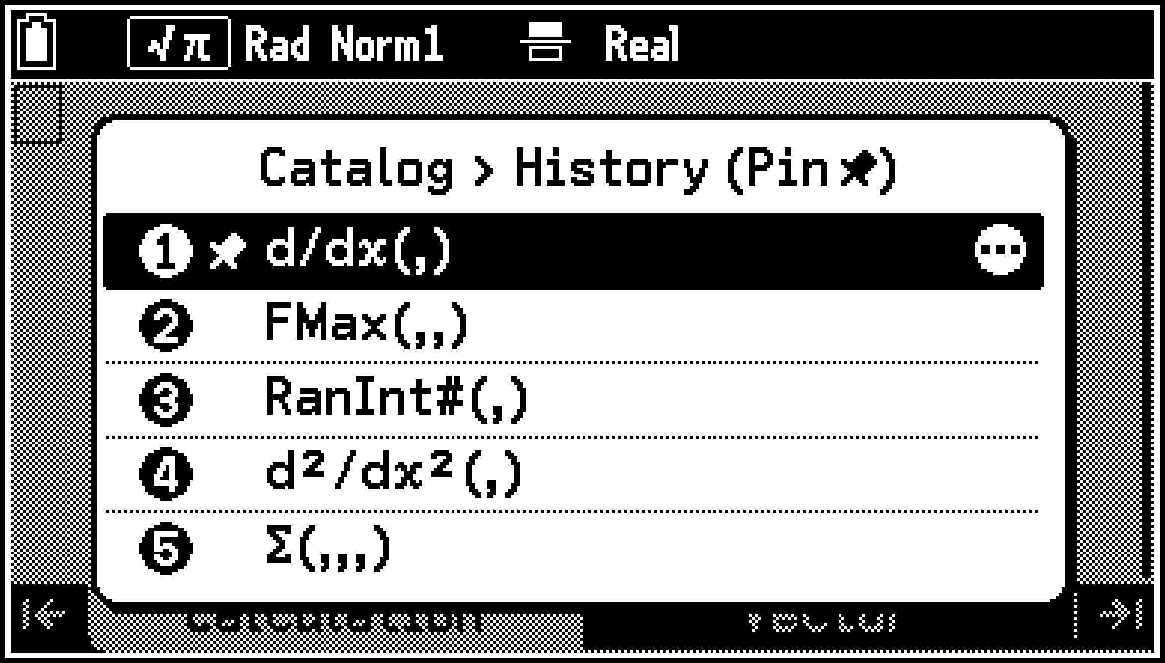
To unpin an item, select the item you wish to unpin and press T.

Category Grouped Item List

Note the following points concerning the syntax of functions and commands, except those in the Unit Conversions category.

If the natural input syntax and line input syntax are different for a function, the natural input syntax is shown first, followed by the line input syntax.

Anything that is optional in a syntax is enclosed in square brackets ([ ]). With the syntax $∫ (f (x), a, b [, t o l])$ , the $t o l$ argument can be omitted, resulting in $∫ (f (x), a, b)$ .

Note

The categories listed in this section and the functions, commands, app variables,^* and symbols included in each category are presented in the order they appear when [Country] > [International] is selected in the System app.

Regardless of the model (fx-CG100 or fx-1AU GRAPH) or configuration, items included in C > [All] are the same. All items listed in this manual are displayed in alphabetical order.

Items included in C > [Variable Data] (input/output variables used in an app)

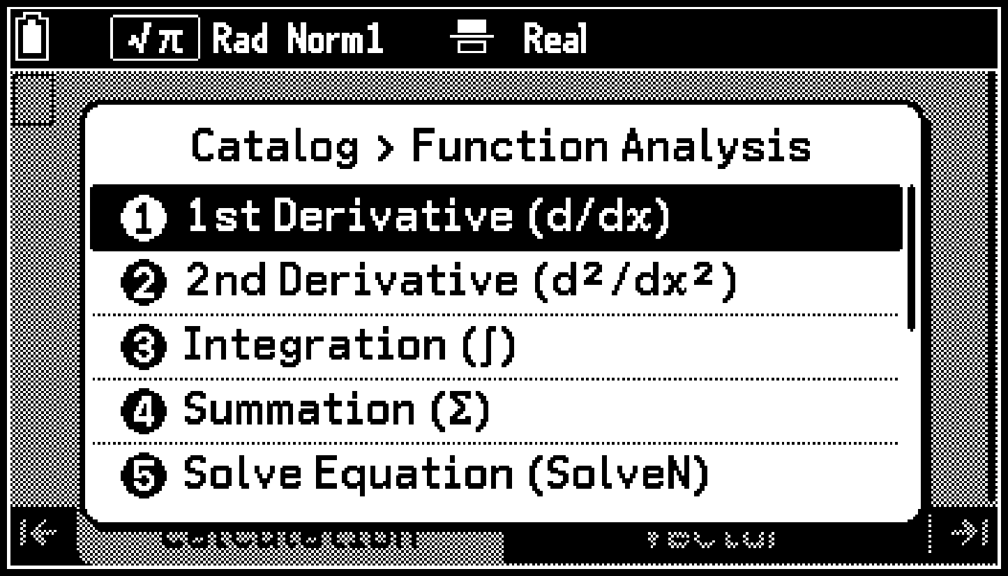
Function Analysis

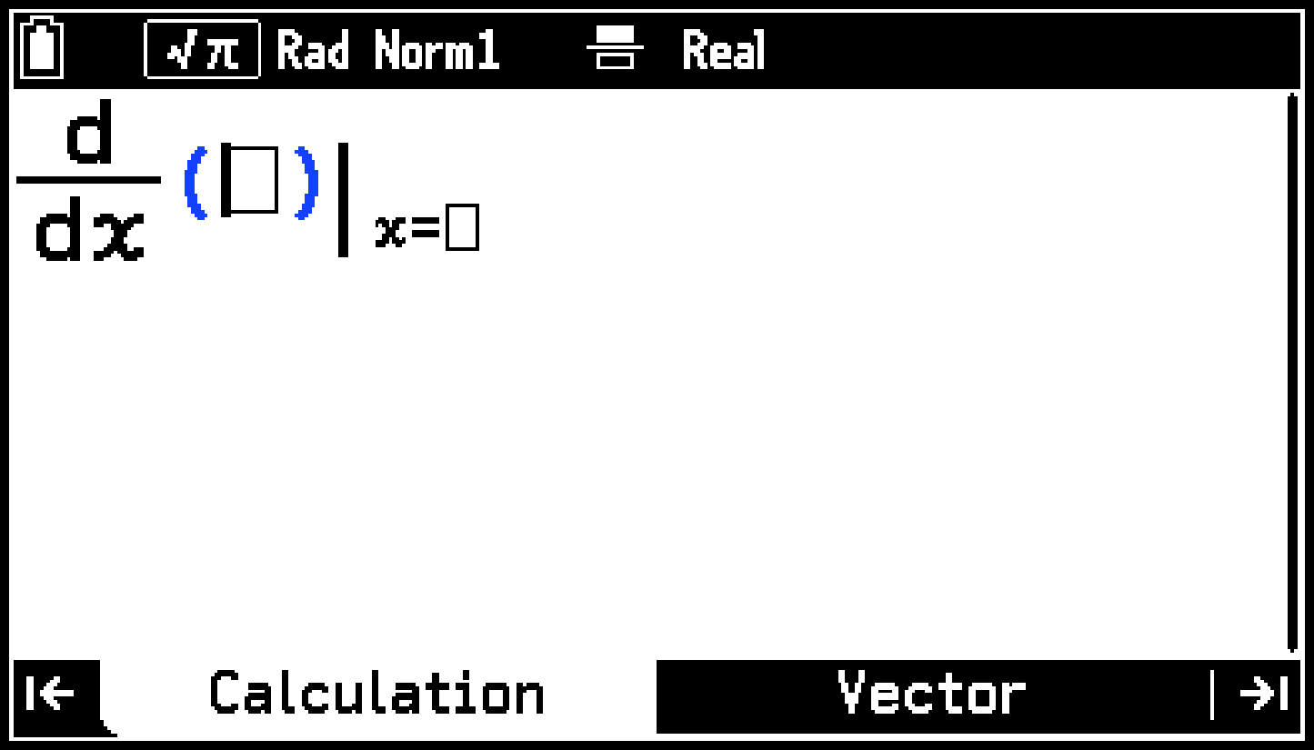
1st Derivative‎ (d/dx) d/dx(,)

Uses approximate calculation to determine the first-order differential coefficient of $f (x)$ at $x = a$ .

Syntax: $\frac{d}{d x} (f (x)) |_{x = a}$ $d / d x (f (x), a)$

Not allowed within this syntax: $d / d x$ , $d^{2} / d x^{2}$ , $∫ d x$ , Σ, FMin, FMax, Solve, RndFix

Example: $\frac{d}{d x} (f (x^{3} + 4 x^{2} + x - 6)) |_{x = 3} = 52$

Precautions

When $f (x)$ is a trigonometric function, make sure to select the following for the angle unit: S > [Angle] > [Radian].

Inaccurate results and errors can be caused by any one of the following:

Discontinuous points in $x$ values

Extreme changes in $x$ values

Inclusion of the local maximum point and local minimum point in $x$ values

Inclusion of the inflection point in $x$ values

Inclusion of indifferentiable points in $x$ values

Calculation results approaching zero

2nd Derivative‎ (d²/dx²) d²/dx²(,)

Uses approximate calculation to determine the second-order differential coefficient of $f (x)$ at $x = a$ .

Syntax: $\frac{d^{2}}{{d x}^{2}} (f (x)) |_{x = a}$ $d^{2} / {d x}^{2} (f (x), a)$

The items that are not allowed within this syntax and precautions are the same as those for $d / d x$ .

Integration‎ (∫)‎ ∫(,,)

Uses approximate calculation to determine the integral of $f (x)$ at $a$ ≤ $x$ ≤ $b$ . This function returns a positive value when $f (x)$ is in the positive range and a negative value when $f (x)$ is in the negative range (Example: $∫_{2}^{3} x^{2} - 4 d x = \frac{7}{3}$ ; $∫_{1}^{2} x^{2} - 4 d x = - \frac{5}{3}$ ).

Syntax: $∫_{a}^{b} f (x) d x$ $∫ (f (x), a, b [, t o l])$

For $t o l$ , input the allowable error (tolerance) range. Default: 1 × 10^-5 if omitted and for natural input.

Not allowed within this syntax: $d / d x$ , $d^{2} / d x^{2}$ , $∫ d x$ , Σ, FMin, FMax, Solve, RndFix

Example: $∫_{1}^{5} {2 x}^{2} + 3 x + 4 d x = \frac{404}{3}$

Precautions

When $f (x)$ is a trigonometric function, make sure to select the following for the angle unit: S > [Angle] > [Radian].

Because numerical integration is used, large error may result in calculated integration values due to the content of $f (x)$ , positive and negative values within the integration interval, or the interval being integrated. (Examples: When there are parts with discontinuous points or abrupt change. When the integration interval is too wide.) In such cases, dividing the integration interval into multiple parts and then performing calculations may improve calculation accuracy.

Summation‎ (Σ) Σ(,,,)

Obtains the sum for a specified range of $f (x)$ .

Syntax: $\sum_{x = a}^{b} (f (x))$ $\sum (f (x), x, a, b [, n])$ $a$ , $b$ , $n$ = integers, $a$ < $b$

$x$ can be any alpha variable. $n$ specifies the step interval. Default: 1 if omitted and for natural input.

Not allowed within this syntax: $d / d x$ , $d^{2} / d x^{2}$ , $∫ d x$ , Σ, FMin, FMax, Solve, RndFix

Example: $\sum_{x = 2}^{6} (x^{2} - 3 x + 5) = 55$

Solve Equation (SolveN) SolveN()

Obtains multiple solutions of an equation.

Syntax: SolveN( $f (x)$ [= right side] [, $x$ ] [,lower limit,upper limit])

If [=right side] is omitted, $f (x)$ = 0 is assumed. Specify any alpha variable for [ $, x$ ] and use the same variable for $f (x)$ . If [, $x$ ] is omitted, the variable $x$ is used.

Up to 10 solutions are returned in list form.

“No Solution” is returned if no solution exists.

If a solution other than one(s) provided might exist, the message “More solutions may exist.‎ ” appears on the display.

Not allowed within this syntax: $d^{2} / d x^{2}$ , Σ, FMin, FMax, Solve

Example: SolveN $(x^{2} - 5 x - 6) = {- 1, 6}$

Solve Equation (Solve) Solve(,)

Approximates a single solution for $f (x)$ = 0. This function has the same functionality as the Equation app’s Using Solver.

Syntax: Solve( $f (x)$ ,initial estimate [,lower limit,upper limit])

Not allowed within this syntax: $d^{2} / d x^{2}$ , Σ, FMin, FMax, Solve

Remainder of Integer‎÷‎Integer Rmdr

Obtains the remainder when an integer is divided by another integer.

Syntax: dividend Rmdr divisor

Example: 17 Rmdr 7 = 3

Integer Part of Int‎÷‎Int Int÷

Obtains the quotient of an integer divided by another integer.

Syntax: dividend Int÷ divisor

Example: 17 Int÷ 7 = 2

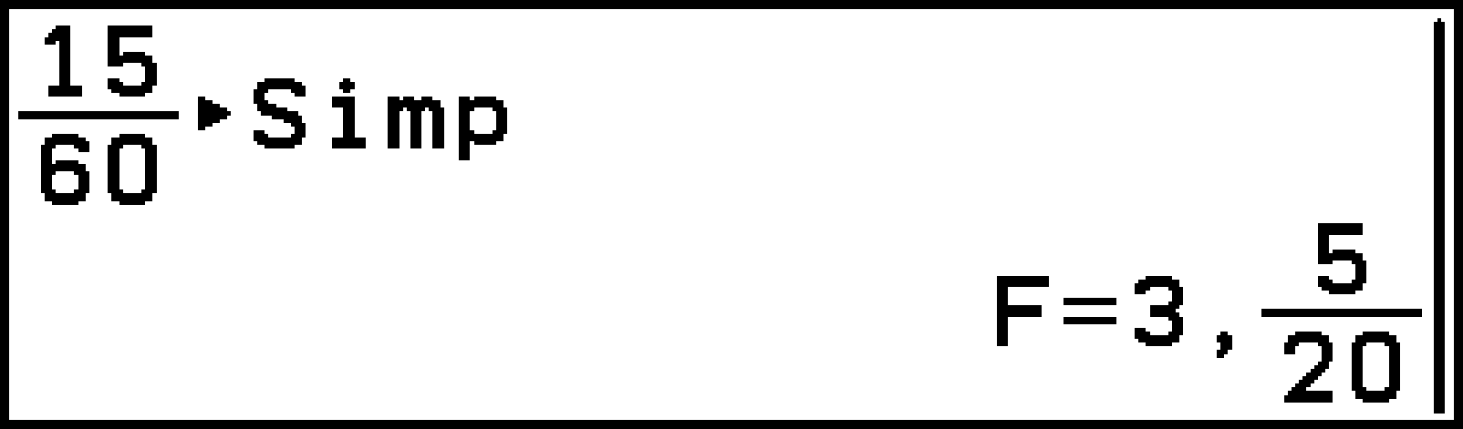
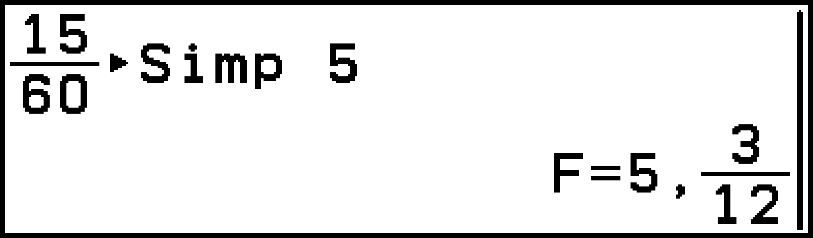
Simplification ISimp

Reduces a fraction to its lowest terms. With the Calculate application, use the settings below.

S > [Simplify] > [Manual]

S > [Complex Mode] > [Real]

Use one of the syntaxes below for ISimp.

Syntax 1: FractionISimp

Automatically reduces the fraction in the argument by dividing by the smallest prime number that can be divided. The prime number and the result of the reduction are shown on the display.

Syntax 2: FractionISimp $n$

Divides the fraction in the argument by the divisor specified by $n$ . The result of the division is shown on the display.

Example 1: $\frac{15}{60} = \frac{5}{20} = \frac{1}{4}$

15e60r
C > [Function Analysis] > [Simplification]E

CY875_Function Analysis_Simplification_1

C > [History (Pin ‎ Pin )‎] > [ISimp]E

CY875_Function Analysis_Simplification_2

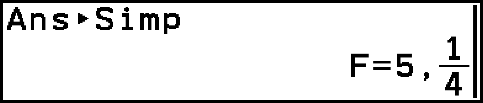
Example 2: $\frac{15}{60} = \frac{3}{12}$ (Specifies a divisor of 5.)

15e60r
C > [Function Analysis] > [Simplification]5E

CY875_Function Analysis_Simplification_3

Precautions

When [a‎+‎b‎ $i$ ‎] or [r‎∠‎θ‎] is selected for S > [Complex Mode], fraction calculation results always are simplified before being displayed, even if S > [Simplify] is set to [Manual].

Function Minimum FMin(,,)

Returns, in list form, the coordinates of the minimum values of $f (x)$ at $a$ ≤ $x$ ≤ $b$ .

Syntax: FMin( $f (x)$ , $a$ , $b$ [, $n$ ]) $n$ : Calculation accuracy ( $n$ = integer from 1 to 9)

Not allowed within this syntax: $d / d x$ , $d^{2} / d x^{2}$ , $∫ d x$ , Σ, FMin, FMax, Solve, RndFix

Example: FMin( $x^{2}$ ,-2,1) = {0,0}

Precautions

Discontinuous points or sections with drastic fluctuation can adversely affect precision or cause an error.

Inputting a larger value for $n$ increases the precision of the calculation, but it also increases the amount of time required to perform the calculation.

Function Maximum FMax(,,)

Returns, in list form, the coordinates of the maximum values of $f (x)$ at $a$ ≤ $x$ ≤ $b$ .

Syntax: FMax( $f (x)$ , $a$ , $b$ [, $n$ ]) $n$ : Calculation accuracy ( $n$ = integer from 1 to 9)

The items that are not allowed within this syntax and precautions are the same as those for FMin.

Probability

Factorial (!)‎ !

Obtains the factorial of 0 or a positive integer.

Syntax: $n!$ $n$ = integer

Permutation‎ (P) P

Obtains the total number of $r$ -permutations taken from set $n$ .

Syntax: $n$ P $r$ $n$ , $r$ = integers

Combination‎ (C) C

Obtains the total number of $r$ -combinations from set $n$ .

Syntax: $n$ C $r$ $n$ , $r$ = integers

Random Number (0 to 1) Ran#

Each execution returns a 10 digit random number (from 0 to 1).

Syntax: Ran# [ $a$ ] 1 ≤ $a$ ≤ 9 ( $a$ = integer)

$a$ : Specifies the random number sequence. If omitted, a true random number is returned. If specified, the corresponding calculator random number sequence is invoked, and a fixed random number is returned. For example, executing Ran# 1 after initializing the sequences^* always returns random numbers from Sequence 1 in order (0.701320948, 0.9297706456, 0.2939058016, ...)

To initialize the sequences, execute Ran# 0. This also initializes the sequences in RanList#. The sequences can also be initialized by using Ran# or RanList# to generate a series of random numbers that is different from the last executed series or by generating a true random number.

Random Integer (n to m) RanInt#(,)

Generates an integer random number between two specified integers $n$ and $m$ .

Syntax: RanInt#( $n$ , $m$ [, $a$ ]) $n$ < $m$ , | $n$ | < 1×10¹⁰, | $m$ | < 1×10¹⁰, $m$ ‒ $n$ < 1×10¹⁰, 1 ≤ $a$ ≤ 999

$a$ : Specifies the number of random numbers. If omitted, one random number is returned. If specified, returns the specified number of random numbers in list form.

Random Number (Normal) RanNorm#(,)

Uses normal distribution to generate a 10-digit random number based on the specified mean $μ$ and standard deviation $σ$ .

Syntax: RanNorm#( $σ$ , $μ$ [, $n$ ]) $σ$ > 0, 1 ≤ $n$ ≤ 999

$n$ : Specifies the number of random numbers. If omitted, one random number is returned. If specified, returns the specified number of random numbers in list form.

Example: To generate a random number of height values obtained according to a normal distribution for a group of children less than one year old with a mean height of 68 cm. Assume that the standard deviation is 8: RanNorm#(8,68)

Random Number (Binomial) RanBin#(,)

Uses binomial distribution based on the specified number of trials $n$ , and the value of probability $p$ to generate a random integer.

Syntax: RanBin#( $n$ , $p$ [, $m$ ]) 1 ≤ $n$ ≤ 100000, 1 ≤ $m$ ≤ 999, 0 ≤ $p$ ≤ 1

$m$ : Specifies the number of random numbers. If omitted, one random number is returned. If specified, returns the specified number of random numbers in list form.

Random Num (0 to 1) to List RanList#()

Each execution returns, in list form, the specified number of random numbers (0 to 1, 10 digits).

Syntax: RanList#( $n$ [, $a$ ]) 1 ≤ $a$ ≤ 9, 1 ≤ $n$ ≤ 999 ( $a$ , $n$ = integers)

$n$ : Specifies the number of trials. This parameter specifies the number of random numbers to be generated.

$a$ : Same as Ran#.

Example: (Immediately after Ran# 0 is executed) RanList#(3,1) = {0.701320948,0.9297706456,0.2939058016}

Random Sample from List RanSamp#(,)

Randomly samples elements from a list and returns the result in list form.

Syntax: RanSamp#(List, $n$ [, $m$ ])

List: A list variables (List 1 through List 26 or List Ans)^* or a list

List variables can also be specified using sub-names.

$n$ : Number of trials (1 ≤ $n$ ≤ 999 when $m$ = 0, 1 ≤ $n$ ≤ number of elements in List when $m$ = 1)

$m$ : Specifies 0 or 1 (0 when omitted). When $m$ = 0, each element can be extracted multiple times. When $m$ = 1, each element can be extracted only once.

Example: To extract two random elements from {1,3,6,7}: RanSamp#({1,3,6,7},2,1)
To extract five random elements from {1,3,6,7}: RanSamp#({1,3,6,7},5)

Numeric Calc

GCD GCD(,)

Obtains the greatest common divisor of multiple integers.

Syntax: GCD( $n$ , $m$ )

LCM LCM(,)

Obtains the least common multiple of multiple integers.

Syntax: LCM( $n$ , $m$ )

Absolute Value Abs()

Finds the absolute value of argument $n$ .

Syntax: | $n$ | Abs( $n$ )

Integer Part Int()

Extracts the integer part of argument $n$ .

Syntax: Int( $n$ )

Example: Int(-3.5) = -3

Fraction Part Frac()

Extracts the fractional part of argument $n$ .

Syntax: Frac( $n$ )

Example: Frac(-3.5) = -0.5

Round Off Rnd

This function is available on the Calculation tab of the Calculate app. It rounds the value of the last calculation result (Ans) on the result display in accordance with the S > [Display] setting.

Syntax: Rnd (no argument, valid for previous calculation result only)

Example: While [Display] > [Fix3: 0.123], to divide 10 by 3 and then multiply Ans by 3

Rnd not used:

10*3E
/3E

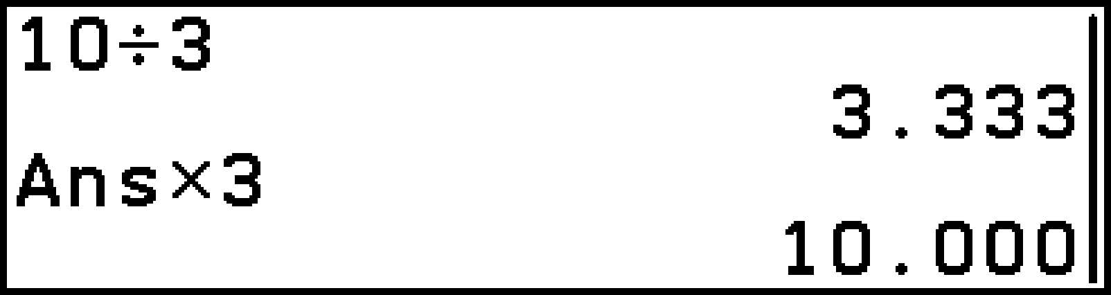
Rnd used:

10*3E
C > [Numeric Calc] > [Round Off]E
/3E

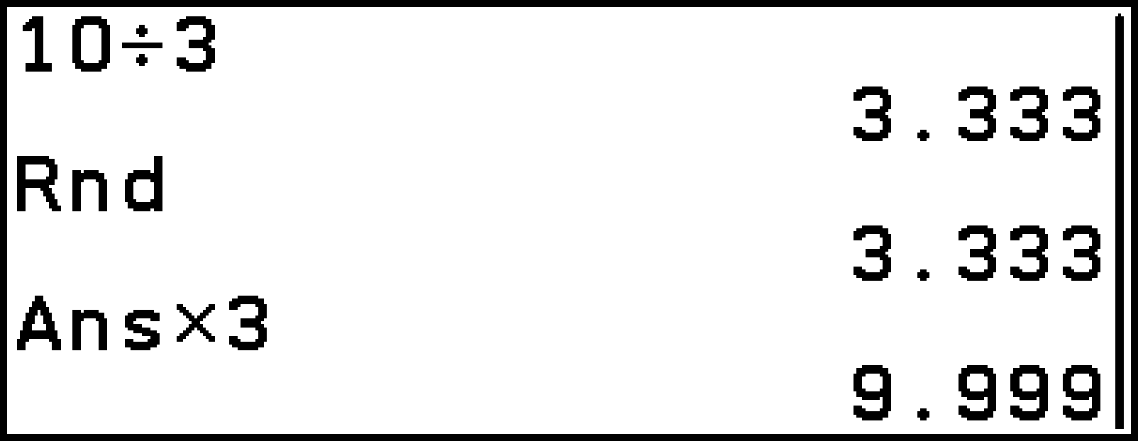
When the setting is [Display] > [Fix3: 0.123], 10÷3=3.333 is displayed, but 15 digits is retained internally, so Ans×3=10.000. If the result of 10÷3 is rounded using Rnd as shown, Ans×3=9.999.

Largest Integer Intg()

Returns the largest integer that does not exceed argument $n$ .

Syntax: Intg( $n$ )

Example: Intg(-10.56) = -11

Round Internal RndFix()

Rounds argument $n$ to the place following the number of decimal places specified by $m$ (0 to 9).

Syntax: RndFix( $n$ [, $m$ ])

If $m$ is omitted, rounding is performed in accordance with the S > [Display] setting, the same as with the Rnd function.

Not allowed within this syntax: $d / d x$ , $d^{2} / d x^{2}$ , $∫ d x$ , Σ, FMin, FMax, Solve, RndFix, logab

Example: RndFix(1.23456,3) = 1.235

Division Remainder MOD(,)

This function obtains the remainder of a division operation. It returns the remainder when $n$ is divided by $m$ .

Syntax: MOD( $n$ , $m$ ) ( $n$ , $m$ = integers)

Example: MOD(17,3) = 2

Remainder Exponentiation MOD_Exp(,,)

This function calculates a modular exponent. It returns the remainder when $n$ is multiplied by $p$ power and then divided by $m$ .

Syntax: MOD_Exp( $n$ , $p$ , $m$ ) ( $n$ , $p$ , $m$ = integers)

Example: MOD(2,4,3) = 1

Vector

Vct $n$ and Vct $m$ can be vectors or vector variables.

The vectors listed the example (such as $[\begin{matrix} 1 & 2 \end{matrix}]$ ) are entered using T > [m×n]. For details, see Inputting a Vector into a Calculation.

Note

When calculating a dot product, cross product, and angle formed by two vectors, the dimensions of the two vectors must be the same.

Vector Vct

Enters “Vct ”. Next, specify a vector variable by entering a letter from A to Z, or Ans.

Dot Product DotP(,)

Obtains the dot product of two vectors.

Syntax: DotP(Vct $n$ ,Vct $m$ )

Example: DotP( $[\begin{matrix} 1 & 2 \end{matrix}]$ , $[\begin{matrix} 3 & 4 \end{matrix}]$ ) = 11

Cross Product CrossP(,)

Obtains the cross product of two vectors.

Syntax: CrossP(Vct $n$ ,Vct $m$ ) (The dimensions of Vct $n$ and Vct $m$ must be 1 × 2, 1 × 3, 2 × 1, or 3 × 1.)

Example: CrossP( $[\begin{matrix} 1 & 2 \end{matrix}]$ , $[\begin{matrix} 3 & 4 \end{matrix}]$ ) = $[\begin{matrix} 0 & 0 & - 2 \end{matrix}]$

‎2-Vector Angle Angle(,)

Obtains the angle between two vectors.

Syntax: Angle(Vct $n$ ,Vct $m$ )

Example: When S > [Angle] > [Radian], Angle( $[\begin{matrix} 1 & 1 \end{matrix}]$ , $[\begin{matrix} - 1 & 1 \end{matrix}]$ ) = $\frac{1}{2} π$

Unit Vector UnitV()

Calculates the unit vector of the vector specified by the argument.

Syntax: UnitV(Vct $n$ )

Example: UnitV( $[\begin{matrix} 5 & 5 \end{matrix}]$ ) = $[\begin{matrix} \frac{\sqrt{2}}{2} & \frac{\sqrt{2}}{2} \end{matrix}]$

Vector Norm Norm()

Calculates the norm (magnitude) of a specified vector or matrix.

Syntax: Norm(Vct $n$ ) ; Norm(Mat $n$ ) (Mat $n$ = matrix or matrix variable)

Example: Norm( $[\begin{matrix} 1 & 3 \end{matrix}]$ ) = $\sqrt{10}$ ; Norm( $[\begin{matrix} 1 & 3 \\ 2 & 4 \end{matrix}]$ ) = $\sqrt{30}$

Matrix

Mat $n$ and Mat $m$ are matrices or matrix variables.

The matrices shown in the example (such as $[\begin{matrix} 0 & - 1 \\ 1 & 0 \end{matrix}]$ ) are entered using T > [m×n]. For details, see Inputting a Matrix into a Calculation.

Note

Determinants and inverse matrices are subject to error due to dropped digits.

The row echelon form and reduced row echelon form operation may not produce accurate results due to dropped digits.

Matrix Mat

Enters “Mat ”. Next, enter a letter from A to Z or Ans to specify a matrix variable.

Inverse Matrix ^-1

Obtains the inverse of the specified square matrix.

Syntax: Mat $n^{- 1}$

Example: ${[\begin{matrix} 0 & - 1 \\ 1 & 0 \end{matrix}]}^{- 1}$ = $[\begin{matrix} 0 & 1 \\ - 1 & 0 \end{matrix}]$

Precautions

Calculation precision is affected for matrices whose determinant is near zero.

Determinant Det()

Obtains the determinant of the specified square matrix.

Syntax: Det(Mat $n$ )

Example: Det( $[\begin{matrix} 1 & 3 \\ 2 & 4 \end{matrix}]$ ) = -2

Matrix Transpose Trn()

Obtains the transpose matrix of the specified matrix.

Syntax: Trn(Mat $n$ )

Example: Trn( $[\begin{matrix} 1 & 2 \\ 3 & 4 \\ 5 & 6 \end{matrix}]$ ) = $[\begin{matrix} 1 & 3 & 5 \\ 2 & 4 & 6 \end{matrix}]$

Note

The “Trn” command can be used with a vector as well. It converts a 1-row × $n$ -column vector to an $n$ -row × 1-column vector, or an $m$ -row × 1-column vector to a 1-row × $m$ -column vector.

Matrix Identity Identity()

Creates an identity matrix with the specified number of rows and columns.

Syntax: Identity( $n$ ) ( $n$ = integer)

Example: Identity(2) = $[\begin{matrix} 1 & 0 \\ 0 & 1 \end{matrix}]$

Row Echelon Form Ref()

This command uses the Gaussian elimination algorithm to find the row echelon form of a matrix.

Syntax: Ref(Mat $n$ )

Example: Ref( $[\begin{matrix} 1 & 2 & 3 \\ 4 & 5 & 6 \end{matrix}]$ ) = $[\begin{matrix} 1 & \frac{5}{4} & \frac{3}{2} \\ 0 & 1 & 2 \end{matrix}]$

Reduced Row Echelon Form Rref()

Obtains the reduced row echelon form of the specified matrix.

Syntax: Rref(Mat $n$ )

Example: Rref( $[\begin{matrix} 1 & 3 & 5 \\ 2 & 4 & 6 \end{matrix}]$ ) = $[\begin{matrix} 1 & 0 & - 1 \\ 0 & 1 & 2 \end{matrix}]$

Matrix Augment Augment(,)

Combines two matrices (or vectors), each of which contains the same number of rows, into a single matrix.

Syntax: Augment(Mat $m$ ,Mat $n$ ) ; Augment(Vct $m$ ,Vct $n$ )

Either or both of the matrices (Mat $m$ , Mat $n$ ) can be replaced with Vct $m$ , Vct $n$ , respectively.

Example: Augment( $[\begin{matrix} 1 & 3 \\ 2 & 4 \end{matrix}]$ , $[\begin{matrix} 2 & 6 \\ 4 & 8 \end{matrix}]$ ) = $[\begin{matrix} 1 & 3 & 2 & 6 \\ 2 & 4 & 4 & 8 \end{matrix}]$ ; Augment( $[\begin{matrix} 1 \\ 2 \end{matrix}]$ , $[\begin{matrix} 2 & 6 \\ 4 & 8 \end{matrix}]$ ) = $[\begin{matrix} 1 & 2 & 6 \\ 2 & 4 & 8 \end{matrix}]$

Fill Matrix Fill(,)

Replaces all elements in a matrix variable (or vector variable) with the specified value $m$ .

Syntax: Fill( $m$ ,Mat $n$ ) ; Fill( $m$ ,Vct $n$ )

Dimensions Dim()

Obtains the dimensions of a matrix (or vector) and outputs them in list form.

Syntax 1: Dim(Mat $n$ ) ; Dim(Vct $n$ )

Since the result of the Dim command is a list, it is stored in List Ans.

Specifies dimensions in list form and creates a matrix (or vector) with all zero elements.

Syntax 2: { $a$ , $b$ } → Dim(Mat $n$ )　( $a$ , $b$ = integers, 1 ≤ $a$ ≤ 999, 1 ≤ $b$ ≤ 999) ;

{ $a$ , $b$ } → Dim(Vct $n$ )　( $a$ , $b$ = integers, 1 ≤ $b$ ≤ 999 when $a$ = 1, 1 ≤ $a$ ≤ 999 when $b$ = 1)

Complex Number

The letter $z$ in the syntax below represents a complex number. Calculations using Arg, Ir∠θ, and Ia+b $i$ are affected by the S > [Angle] setting.

Note

The calculator regards a complex number in the form a+b $i$ as a coordinate on a Gaussian plane, and calculates absolute value | $z$ | and argument Arg( $z$ ).

Norm of a Complex Number Abs()

Obtains the absolute value of a complex number.

Syntax: | $z$ | Abs( $z$ )

Example: |1+ $i$ | = $\sqrt{2}$

Argument Arg()

Obtains the argument of a complex number.

Syntax: Arg( $z$ )

Example: Arg(1+ $i$ ) = $\frac{1}{4} π$ (S > [Angle] > [Radian])

Complex Conjugate Conjg()

Obtains the conjugate complex number.

Syntax: Conjg( $z$ )

Example: Conjg(1+ $i$ ) = 1 $- i$

Real Part ReP()

Extracts the real part of a complex number.

Syntax: ReP( $z$ )

Example: ReP(1+2 $i$ ) = 1

Imaginary Part ImP()

Extracts the imaginary part of a complex number.

Syntax: ImP( $z$ )

Example: ImP(1+2 $i$ ) = 2

Ir∠θ Ir∠θ

Converts a rectangular form value to polar form.

Syntax: $z$ Ir∠θ

Example: $1 + \sqrt{3} i$ Ir∠θ = 2∠ $\frac{1}{3} π$ (S > [Angle] > [Radian])

Ia+b $i$ Ia+b $i$

Converts a polar form to rectangular form.

Syntax: $z$ Ia+b $i$

Example: 2∠ $\frac{1}{3} π$ Ia+b $i$ = $1 + \sqrt{3} i$ (S > [Angle] > [Radian])

Statistics

In all of the syntaxes below, “List $n$ ” and “List $m$ ” are lists or list variables. For list variables, $n$ , $m$ can be a value from 1 to 26, or Ans. List variables can also be specified using sub-names.

{} {}

Inputs curly brackets ( { } ) to enter a new list.

List List

Inputs “List ”. Following “List ”, input a value from 1 to 26, or Ans to specify a list variable.

Dimensions Dim()

Determines the number of elements in a list.

Syntax 1: Dim(List $n$ )

Specifies the number of list elements and creates a list variable with zero in all elements.

Syntax 2: Number of Elements $a$ → Dim(List $n$ ) ( $a$ = integer, 1 ≤ $a$ ≤ 999)

Fill List Fill(,)

Replaces the values in all elements in a list variable with the same value ( $a$ ).

Syntax: Fill( $a$ ,List $n$ )

Generate Sequence Seq(,,,,)

Defines a function to generate a number sequence and return it in list form.

Syntax: Seq( $f (x)$ , $x$ ,Start Value,End Value,Increment)

$x$ can be any alpha variable.

Example: Seq( $x^{2}$ , $x$ ,1,11,5) = {1,36,121}

Minimum Min()

Syntax 1: Min(List $n$ ) Extracts the minimum value from all elements in a list.

Syntax 2: Min(List $n$ ,List $m$ ) Extracts the lesser element at the same position in two lists.

Maximum Max()

Syntax 1: Max(List $n$ ) Extracts the maximum value from all elements in a list.

Syntax 2: Max(List $n$ ,List $m$ ) Extracts the larger element at the same position in two lists.

Mean Mean()

Finds the mean value of all elements in a list.

Syntax: Mean(List $n$ )

Median Median()

Finds the median of two lists, one of which is data and the other is frequencies.

Syntax: Median(List $n$ ,List $m$ )

List $n$ ： Data list, List $m$ ： Frequency list
The number of elements in List $n$ and List $m$ must be the same.

Example: When List 1 = {36,16,58,46,56}, List 2 = {75,89,98,72,67}, Median(List 1,List 2) = 46

Combine Lists Augment(,)

Combines two lists into one.

Syntax: Augment(List $n$ ,List $m$ )

Sum of List Elements Sum()

Finds the sum of all elements in a list.

Syntax: Sum(List $n$ )

List Product Prod()

Finds the sum product of all the elements in a list.

Syntax: Prod(List $n$ )

Cumulative Frequency Cuml()

Calculates the cumulative frequency of the elements of a list.

Syntax: Cuml(List $n$ )

Example: When List 1 = {2,3,6,5,4}, Cuml(List 1) = {2,5,11,16,20}

Data Percentages Percent()

Calculates the percentage of each element relative to the sum of all elements in a list.

Syntax: Percent(List $n$ )

List Data Diff ΔList

Calculates {Element 2 − Element 1, Element 3 − Element 2, ... Element $n$ − Element $n$ −1} in a list of $n$ ( $n$ ≥ 2) elements and returns the result in list form.

Syntax: ΔList $a$ ( $a$ = List variable number)

Note: You can save the result to List 2 by typing “ΔList 1→List 2”.

Estimated x-Data $\hat{x}$
Estimated y-Data $\hat{y}$

These functions are used immediately after performing a regression calculation^* with the Statistics app. For a value specified for one variable ( $x$ or $y$ ) they, estimate the other variable, based on a regression model.

Syntax: $y$ -value $\hat{x}$ (Calculates an estimated $x$ -value for the $y$ -value.)

$x$ -value $\hat{y}$ (Calculates an estimated $y$ -value for the $x$ -value.)

Estimated values cannot be calculated for the following types of regression model: Med-Med Regression, Quadratic Regression, Cubic Regression, Quartic Regression, Sinusoidal Regression, Logarithm Regression.

Sample Standard Deviation StdDev()

Finds the sample standard deviation of data specified by a list.

Syntax: StdDev(List $n$ [,List $m$ ]) (List $n$ ... Sample data, List $m$ ... Frequency data)

Example: StdDev({10,20,30,40},{3,5,4,1}) = 9.26808696

Population Standard Deviation StdDev_σ()

Finds the population standard deviation of data specified by a list.

Syntax: StdDev_σ(List $n$ [,List $m$ ]) (List $n$ ... Sample data, List $m$ ... Frequency data)

Unbiased Variance Variance()

Finds the unbiased variance of data specified by a list.

Syntax: Variance(List $n$ [,List $m$ ]) (List $n$ ... Sample data, List $m$ ... Frequency data)

Population Variance Variance_ $σ^{2}$ ()

Finds the population variance of data specified by a list.

Syntax: Variance_ $σ^{2}$ (List $n$ [,List $m$ ]) (List $n$ ... Sample data, List $m$ ... Frequency data)

List to Matrix List→Mat()

Saves list contents to Mat Ans.

Syntax: List→Mat(List $n$ ,List $m$ )
(The number of elements in List $n$ and List $m$ must be the same.)

Example: When List 1 = {2,3,4}, List 2 = {20,30,40}, List→Mat(List 1,List 2) = $[\begin{matrix} 2 & 20 \\ 3 & 30 \\ 4 & 40 \end{matrix}]$

Matrix to List Mat→List()

Saves the specified columns of a matrix variable to List Ans.

Syntax: Mat→List(Mat $n$ , $m$ )
( $n$ is a letter from A to Z, or Ans, and $m$ is a column number.)

Example: When Mat A = $[\begin{matrix} 2 & 20 \\ 3 & 30 \\ 4 & 40 \end{matrix}]$ , Mat→List(Mat A,1) = {2,3,4}

Note: You can assign the elements of Column 1 of Mat A to List 1 by inputting “Mat→List(Mat A,1)→List 1”.

Distribution: Probability Calculation for Standard Normal Distribution

Attention fx-1AU GRAPH Users

The fx-1AU GRAPH does not have a Distribution category, but all commands described in this section can be called from C > [All].
Example: To call "P()", select C > [All] > [P] > [P()].

Each mathematical function described in this section is intended for use immediately after you perform a ‎1-Variable statistical calculation with the Statistics app.

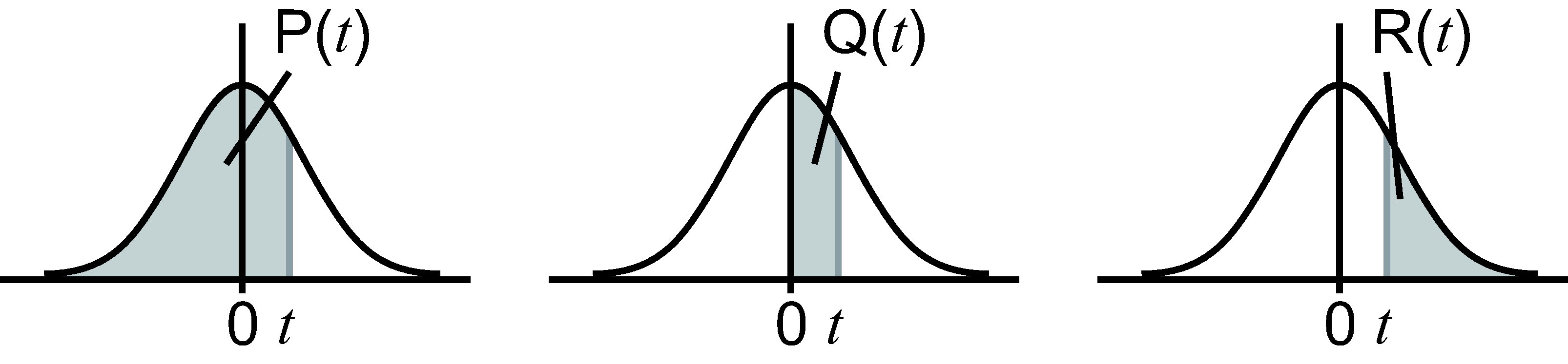
Normal Probability P(t)     P()
Normal Probability‎ Q(t)     Q()
Normal Probability R(t)     R()

Taking normalized variable $t$ as an argument, these functions find the probability values for the standard normal distribution shown in the figures below. The $t$ -value is determined using the function t().

Syntax: P( $t$ ) ; Q( $t$ ) ; R( $t$ )

Normal Variable t(x) t()

Normalized variable t( $x$ ) at data value $x$ is determined using the formula below based on the mean $\bar{x}$ and population standard deviation $σ_{x}$ , which is obtained as the result of ‎1-Variable statistical calculation.

$t (x) = \frac{x - \bar{x}}{σ_{x}}$

Syntax: t( $x$ )

This function is used in combination with P(), Q(), and R() to find the probability values of the standard normal distribution.

Example: The height data of 20 students at a university were input with the Statistics app and a ‎1-Variable statistical calculation was performed. Determine what percentile does the 180 cm tall student fall.

R(t(180))

Distribution: Distribution Calculations

Attention fx-1AU GRAPH Users

The fx-1AU GRAPH does not have a Distribution category, but all commands described in this section can be called from C > [All].
Example: To call "NormPD()", select C > [All] > [N] > [NormPD()].

Each function in this section performs a different type of distribution calculation.

Syntax Notes

The list below shows the meanings of the symbols and abbreviations in the syntax.

$x$ : data value

Lower: lower boundary

Upper: upper boundary

$μ$ ： population mean

$σ$ ： population standard deviation ( $σ$ > 0)

$λ$ ： mean ( $λ$ > 0)

$p$ : probability (0 ≤ $p$ ≤ 1)

df: degrees of freedom (df > 0)

$n$ :df: degrees of freedom of numerator (positive integer)

$d$ :df: degrees of freedom of denominator (positive integer)

$P$ : success probability (0 ≤ $P$ ≤ 1)

$n$ : number of trials from population (0 ≤ $n$ integer)

$M$ : number of successes in population (0 ≤ $M$ integer)

$N$ : population size ( $n$ ≤ $N$ , $M$ ≤ $N$ integer)

The following values are substituted whenever any of the arguments enclosed in brackets ([ ]) are omitted.
$μ$ =0, $σ$ =1, tail=”L” (Left)

Calculation Result Storage Variables

Variables (p, xInv, x1InvN, x2InvN, zLow, zUp, tLow, tUp) to which the calculation results of each function are stored can be accessed from C > [Variable Data] > [Distribution].

Normal Probability Density NormPD()

Returns the normal probability density ( $p$ value) for the specified data.

Syntax: NormPD( $x$ [, $μ$ , $σ$ ])

A single value or a list can be specified for $x$ . Calculation result $p$ is assigned to variables $p$ and Ans (List Ans when $x$ is a list).

Example: NormPD(1) = 0.2419707245 ; NormPD({0.5,1}) = {0.3520653268,0.2419707245}

Normal Cumulative Dist NormCD(,)

Returns the normal cumulative distribution ( $p$ value) for the specified data.

Syntax: NormCD(Lower,Upper[, $μ$ , $σ$ ])

Single values or lists can be specified for Lower and Upper. Calculation results $p$ , zLow, and zUp are assigned respectively to variables $p$ , zLow, and zUp. Calculation result $p$ also is assigned to Ans (List Ans when Lower and Upper are lists).

Example: NormCD(-1,1) = 0.6826894921 ; NormCD({-1,-2},{1,2}) = {0.6826894921,0.9544997361}

Inverse Normal Cumul Dist InvNormCD()

Returns the inverse normal cumulative distribution (Lower and/or Upper value(s)) for the specified $p$ -value.

Syntax: InvNormCD([tail,] $p$ [, $μ$ , $σ$ ])

You can specify Left, Right, or Center for “tail”. To specify the “tail” setting, input the numbers or letters below.

Left： -1 or ”L”

Center： 0 or ”C”

Right： 1 or ”R”

A single value or a list can be specified for $p$ . Calculation results are output in accordance with the tail setting as described below.

tail = Left	The Upper value is assigned to variables x1InvN and Ans (List Ans when $p$ is a list).
tail = Right	The Lower value is assigned to variables x1InvN and Ans (List Ans when $p$ is a list).
tail = Central	The Lower and Upper values are assigned respectively to variables x1InvN and x2InvN. Lower only is assigned to Ans (List Ans when $p$ is a list).

Example: InvNormCD(”L”,0.7,35,2) = 36.04880103
InvNormCD({0.5,0.7},35,2) = {35,36.04880103}

t Probability Density tPD(,)

Returns the Student- $t$ probability density ( $p$ value) for the specified data.

Syntax: tPD( $x$ ,df)

See PD Syntax.

Example: tPD(1,1) = 0.1591549431 ; tPD({0,1},1) = {0.3183098862,0.1591549431}

t Cumulative Distribution tCD(,,)

Returns the Student- $t$ cumulative distribution ( $p$ value) for the specified data.

Syntax: tCD(Lower,Upper,df)

Single values or lists can be specified for Lower and Upper. Calculation results $p$ , tLow, and tUp are assigned respectively to variables $p$ , tLow, and tUp. Calculation result $p$ also is assigned to Ans (List Ans when Lower and Upper are lists).

Example: tCD(0,1,1) = 0.25 ; tCD({0,0},{1,2},1) = {0.25,0.3524163823}

Inverse t Cumulative Dist InvTCD(,)

Returns the inverse Student- $t$ cumulative distribution (Lower value) for the specified $p$ value.

Syntax: InvTCD( $p$ ,df)

See Inverse CD Syntax (continuous distributions).

Example: InvTCD(0.25,1) = 1 ; InvTCD({0.25,0.75},1) = {1,-1}

‎ $χ^{2}$ ‎ Probability Density ChiPD(,)

Returns the $χ^{2}$ probability density ( $p$ value) for the specified data.

Syntax: ChiPD( $x$ ,df)

See PD Syntax.

Example: ChiPD(1,1) = 0.2419707245 ; ChiPD({0,1},1) = {0,0.2419707245}

‎ $χ^{2}$ ‎ Cumulative Distribution ChiCD(,,)

Returns the $χ^{2}$ cumulative distribution ( $p$ value) for the specified data.

Syntax: ChiCD(Lower,Upper,df)

See CD Syntax.

Example: ChiCD(0,1,1) = 0.6826894921 ; ChiCD({0,0},{1,2},1) = {0.6826894921,0.8427007929}

Inverse‎ ‎ $χ^{2}$ Cumulative Dist InvChiCD(,)

Returns the inverse $χ^{2}$ cumulative distribution (Lower value) for the specified $p$ value.

Syntax: InvChiCD( $p$ ,df)

See Inverse CD Syntax (continuous distributions).

Example: InvChiCD(0.319,1) = 0.9930420738 ; InvChiCD({0.64,0.319},1) = {0.2187421667,0.9930420738}

F Probability Density FPD(,,)

Returns the $F$ probability density ( $p$ value) for the specified data.

Syntax: FPD( $x$ , $n$ :df, $d$ :df)

See PD Syntax.

Example: FPD(1,1,2) = 0.1924500897 ; FPD({1,2},1,2) = {0.1924500897,0.08838834765}

F Cumulative Distribution FCD(,,,)

Returns the $F$ cumulative distribution ( $p$ value) for the specified data.

Syntax: FCD(Lower,Upper, $n$ :df, $d$ :df)

See CD Syntax.

Example: FCD(0,1,1,2) = 0.5773502692 ; FCD({0,0},{1,2},1,2) = {0.5773502692,0.7071067812}

Inverse F Cumulative Dist InvFCD(,,)

Returns the inverse $F$ cumulative distribution (Lower value) for the specified $p$ value.

Syntax: InvFCD( $p$ , $n$ :df, $d$ :df)

See Inverse CD Syntax (continuous distributions).

Example: InvFCD(0.43,1,2) = 0.9625240705 ; InvFCD({0.86,0.43},1,2) = {0.03998368013,0.9625240705}

Binomial Probability BinomialPD(,)

Returns the binomial probability ( $p$ value) for the specified data.

Syntax: BinomialPD([ $x$ ,] $n$ , $P$ )

See PD Syntax.

Example: BinomialPD(3,5,0.5) = 0.3125 ; BinomialPD({3,5},5,0.5) = {0.3125,0.03125}

Binomial Cumulative Dist BinomialCD(,)

Returns the binomial cumulative distribution ( $p$ value) for the specified data.

Syntax: BinomialCD([[Lower,]Upper,] $n$ , $P$ )

See CD Syntax.

Example: BinomialCD(5,10,0.5) = 0.623046875 ; BinomialCD({0,5},{5,8},10,0.5) = {0.623046875,0.6123046875}

Inverse Binomial Cumulative Dist InvBinomialCD(,,)

Returns the inverse binomial cumulative distribution for the specified $p$ value.

Syntax: InvBinomialCD( $p$ , $n$ , $P$ )

See Inverse CD Syntax (discrete distributions).

Example: InvBinomialCD(0.6,10,0.5) = 5 ; InvBinomialCD({0.6,0.3},10,0.5) = {5,4}

Precautions

When executing the Inverse Binomial Cumulative Distribution calculation, the calculator uses the specified $p$ value and the value that is one less than the $p$ value minimum number of significant digits ( $p$ ’ value) to calculate minimum number of trials values. The results are assigned to variables xInv (calculation result using $p$ ) and *xInv (calculation result using $p$ ’). The calculator always displays the xInv value only. However, when the xInv and *xInv values are different, the message shown below will appear with both values.

CY875_V2_Catalog Distribution_2 + CY875_V2_Catalog Distribution_2

$p$ value

$p$ ’ value

The calculation results of Inverse Binomial Cumulative Distribution are integers. Accuracy may be reduced when the $p$ value has 10 or more digits. Note that even a slight difference in calculation accuracy affects calculation results. If a warning message appears, check the displayed values.

Poisson Probability PoissonPD(,)

Returns the Poisson probability ( $p$ value) for the specified data.

Syntax: PoissonPD( $x$ , $λ$ )

See PD Syntax.

Example: PoissonPD(1,1.2) = 0.3614330543 ; PoissonPD({1,2},1.2) = {0.3614330543,0.2168598326}

Poisson Cumulative Dist PoissonCD(,)

Returns the Poisson cumulative distribution ( $p$ value) for the specified data.

Syntax: PoissonCD([Lower,]Upper, $λ$ )

See CD Syntax.

If Lower is omitted, Lower = 0 is assumed.

Example: PoissonCD(1,2,1.2) = 0.5782928869 ; PoissonCD({1,1},{2,3},1.2) = {0.5782928869,0.6650368199}

Inverse Poisson Cumul Dist InvPoissonCD(,)

Returns the inverse Poisson cumulative distribution for the specified $p$ value.

Syntax: InvPoissonCD( $p$ , $λ$ )

See Inverse CD Syntax (discrete distributions).

Example: InvPoissonCD(0.58,1.2) = 1 ; InvPoissonCD({0.58,0.75},1.2) = {1,2}

Precautions are the same as those for Inverse Binomial Cumulative Dist.

Geometric Probability GeoPD(,)

Returns the geometric probability ( $p$ value) for the specified data.

Syntax: GeoPD( $x$ , $P$ )

See PD Syntax.

Example: GeoPD(2,0.8) = 0.16 ; GeoPD({2,3},0.8) = {0.16,0.032}

Geometric Cumulative Dist GeoCD(,)

Returns the geometric cumulative distribution ( $p$ value) for the specified data.

Syntax: GeoCD([Lower,]Upper, $P$ )

See CD Syntax.

If Lower is omitted, Lower = 0 is assumed.

Example: GeoCD(1,2,0.8) = 0.96 ; GeoCD({1,1},{2,3},0.8) = {0.96,0.992}

Inverse Geometric Cumul Dist InvGeoCD(,)

Returns the inverse geometric cumulative distribution for the specified $p$ value.

Syntax: InvGeoCD( $p$ , $P$ )

See Inverse CD Syntax (discrete distributions).

Example: InvGeoCD(0.96,0.8) = 2 ; InvGeoCD({0.96,0.992},0.8) = {2,3}

Precautions are the same as those for Inverse Binomial Cumulative Dist.

Hypergeometric Probability HypergeoPD(,,,)

Returns the hypergeometric probability ( $p$ value) for the specified data.

Syntax: HypergeoPD( $x$ , $n$ , $M$ , $N$ )

See PD Syntax.

Example: HypergeoPD(1,5,10,20) = 0.1354489164 ; HypergeoPD({1,2},5,10,20) = {0.1354489164,0.3482972136}

Hypergeometric Cumul Dist HypergeoCD(,,,)

Returns the hypergeometric cumulative distribution ( $p$ value) for the specified data.

Syntax: HypergeoCD([Lower,]Upper, $n$ , $M$ , $N$ )

See CD Syntax.

If Lower is omitted, Lower = 0 is assumed.

Example: HypergeoCD(1,2,5,10,20) = 0.48374613 ; HypergeoCD({1,1},{2,3},5,10,20) = {0.48374613,0.8320433437}

Inverse Hypergeo Cumul Dist InvHypergeoCD(,,,)

Returns the inverse hypergeometric cumulative distribution for the specified $p$ value.

Syntax: InvHypergeoCD( $p$ , $n$ , $M$ , $N$ )

See Inverse CD Syntax (discrete distributions).

Example: InvHypergeoCD(0.48,5,10,20) = 2 ; InvHypergeoCD({0.48,0.83},5,10,20) = {2,3}

Precautions are the same as those for Inverse Binomial Cumulative Dist.

Syntax and description

Syntax	Description
PD Syntax	A single value or a list can be specified for $x$ . Calculation result $p$ is assigned to variables $p$ and Ans (List Ans when $x$ is a list).
CD Syntax	Single values or lists can be specified for Lower and Upper. Calculation result $p$ is assigned to variables $p$ and Ans (List Ans when Lower and Upper are lists).
Inverse CD Syntax (continuous distributions)	A single value or a list can be specified for $p$ . The Lower value is assigned to the xInv and Ans variables (List Ans when $p$ is a list).
Inverse CD Syntax (discrete distributions)	A single value or a list can be specified for $p$ . The calculation result X value is assigned to the xInv and Ans variables (List Ans when $p$ is a list).

Angle/Coord/Sexa

Degrees °

Specifies degrees as the angle unit.

Syntax: $n$ °

Example: When S > [Angle] > [Radian], 90° = $\frac{1}{2} π$

Radians $^{r}$

Specifies radians as the angular unit.

Syntax: $n^{r}$

Example: When S > [Angle] > [Degree], $\frac{π}{2}^{r}$ = 90

Gradians $^{g}$

Specifies gradians as the angle unit.

Syntax: $n^{g}$

Example: When S > [Angle] > [Degree], $100^{g}$ = 90

Rectangular to Polar Pol(,)

Converts rectangular coordinate values to polar coordinates and returns them in list form.

Syntax: Pol( $x$ , $y$ ) = ( $r$ , $θ$ )

The resulting polar coordinates $θ$ are displayed in the range as follows, depending on the S > [Angle] setting.

Degree: -180 < $θ$ ≤ 180

Radian: - $π$ < $θ$ ≤ $π$

Gradian: -200 < $θ$ ≤ 200

Example: When S > [Angle] > [Radian], Pol( $\sqrt{2}$ , $\sqrt{2}$ ) = {2, $\frac{1}{4} π$ }

Polar to Rectangular Rec(,)

Converts polar coordinate values to rectangular coordinates and returns them in list form.

Syntax: Rec( $r$ , $θ$ ) = ( $x$ , $y$ )

Example: When S > [Angle] > [Radian], Rec(2, $\frac{1}{4} π$ ) = { $\sqrt{2}$ , $\sqrt{2}$ }

Degs Mins Secs °

Inputs a sexagesimal value.

Syntax: Degree Value°[Minute Value°[Seconds Value°]]

Example: 1°15° = 1.25 ; 0°75° = 1.25 ; 0°15° = 0.25 ; 0°0°900° = 0.25

Note: To display calculation results as sexagesimal values, select sF > [Sexagesimal]. For more information, see Changing the Display Format of Calculation Results (Format Menu).

Decimal to Sexagesimal IDMS

Converts a decimal value to a sexagesimal value (degrees (hours), minutes, seconds).

Syntax: $n$ IDMS

Example: 1.25IDMS = 1°15’00”

Hyperbolic Calc

Hyperbolic and inverse hyperbolic functions can be input using the menu items below.

Menu item	Function
sinh	sinh()
cosh	cosh()
tanh	tanh()
sinh‎ $^{-1}$ ‎	sinh $^{-1}$ ()
cosh‎ $^{-1}$ ‎	cosh $^{-1}$ ()
tanh‎ $^{-1}$ ‎	tanh $^{-1}$ ()

Example: sinh(1) = 1.175201194 ; sinh $^{-1}$ (Ans) = 1

Engineer Symbol

Engineering symbols can be input using the menu items below.

Menu item	Symbol	$10^{n}$
Milli	m	$10^{-3}$
Micro	μ	$10^{-6}$
Nano	n	$10^{-9}$
Pico	p	$10^{-12}$
Femto	f	$10^{-15}$
Kilo	k	$10^{3}$
Mega	M	$10^{6}$
Giga	G	$10^{9}$
Tera	T	$10^{12}$
Peta	P	$10^{15}$
Exa	E	$10^{18}$

Appending an engineering symbol immediately after a value causes the value to be $10^{n}$ (where $n$ is an integer multiple of 3).

Example: 7.1k = 7100 ; 2G÷100M = 20

Note: To display calculation results with engineering symbols, turn on S > [Display] > [Engineer Symbol]. For details, see Display (General).

Unit Conversions

Converts a value of one unit to a different unit.

Syntax: $n$ unit command Unit Conversions unit command ( $n$ = real number or list of real numbers)

The two unit commands are linked with “ Unit Conversions ” and used as a single unit conversion command. The two unit commands must be from the same category. Refer to the “Unit Command List” below for available unit commands.

Example: 25.4 [cm] Unit Conversions [in] = 10 ; {175,162} [m²] [ha] = {0.0175,0.0162}

Unit Command List

Category	Unit Command
Length	[fm]
	[Å]
	[μm]
	[mm]
	[cm]
	[m]
	[km]
	[AU]
	[l.y.]
	[pc]
	[Mil]
	[in]
	[ft]
	[yd]
	[fath]
	[rd]
	[mile]
	[n mile]
Area	[cm²]
	[m²]
	[ha]
	[km²]
	[in²]
	[ft²]
	[yd²]
	[acre]
	[mile²]
Volume	[cm³]
	[mL]
	[L]
	[m³]
	[in³]
	[ft³]
	[fl_oz(UK)]
	[fl_oz(US)]
	[gal(US)]
	[gal(UK)]
	[pt]
	[qt]
	[tsp]
	[tbsp]
	[cup]
Time	[ns]
	[μs]
	[ms]
	[s]
	[min]
	[h]
	[day]
	[week]
	[yr]
	[s-yr]
	[t-yr]
Temperature	[°C]
	[K]
	[°F]
	[°R]
Velocity	[m/s]
	[km/h]
	[knot]
	[ft/s]
	[mile/h]
Mass	[u]
	[mg]
	[g]
	[kg]
	[mton]
	[oz]
	[lb]
	[slug]
	[ton(short)]
	[ton(long)]
Force	[N]
	[lbf]
	[tonf]
	[dyne]
	[kgf]
Pressure	[Pa]
	[kPa]
	[mmH₂O]
	[mmHg]
	[atm]
	[inH₂O]
	[inHg]
	[lbf/in²]
	[bar]
	[kgf/cm²]
Energy	[eV]
	[J]
	[cal_th]
	[cal₁₅]
	[cal_IT]
	[kcal_th]
	[kcal₁₅]
	[kcal_IT]
	[l-atm]
	[kW･h]
	[ft･lbf]
	[Btu]
	[erg]
	[kgf･m]
Power	[W]
	[cal_th/s]
	[hp]
	[ft･lbf/s]
	[Btu/min]

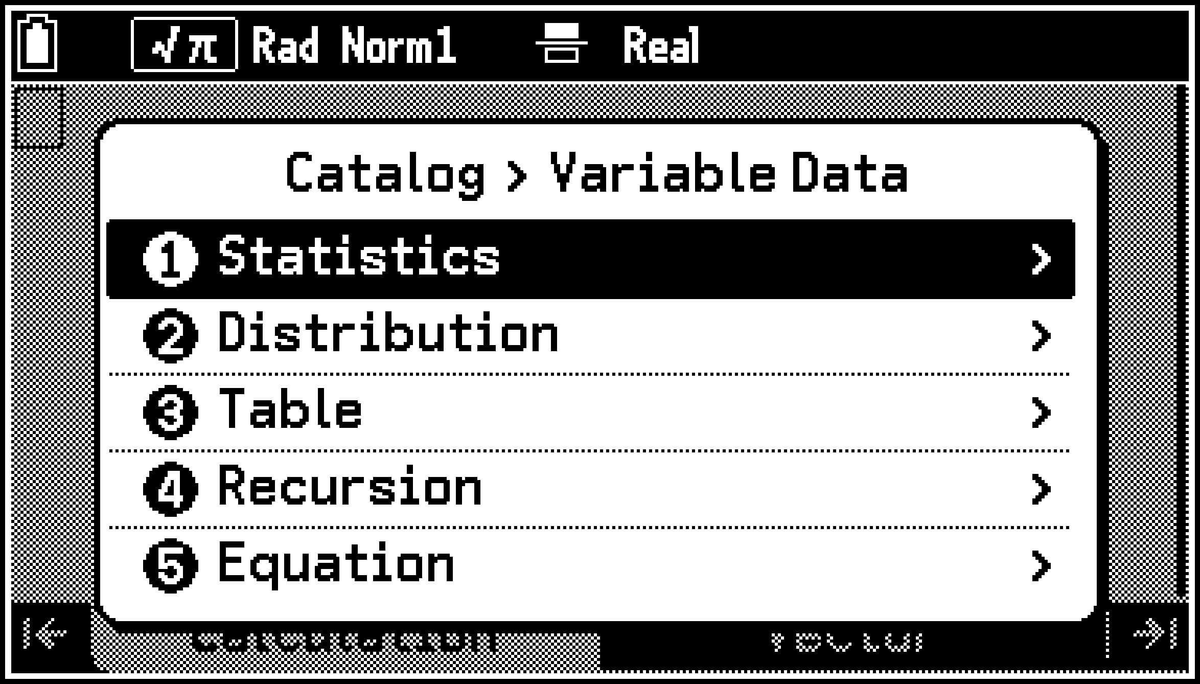
Variable Data

The Variable Data category contains variables that store input and output values of each app. The menu items that appear when you select C > [Variable Data] are app names.

Variable Data > Statistics

Variables in this category store input values and calculation results for statistical calculations performed and graphs drawn using the Statistics app.

Statistics > X

Single-variable or paired-variable statistical calculation $x$ -data values:

Menu item	Variable
Data Items	n
Data x Mean	$\bar{x}$
Data x Sum	$Σ x$
x-Data Sum of Squares	$Σ x^{2}$
x-Data Population Std Dev	σx
x-Data Sample Std Dev	sx
X-Data Minimum	minX
X-Data Maximum	maxX

Statistics > Y

Paired-variable statistical calculation $y$ -data values:

Menu item	Variable
Data y Mean	$\bar{y}$
Data y Sum	$Σ y$
y-Data Sum of Squares	$Σ y^{2}$
xy-Data Products Sum	$Σ xy$
y-Data Population Std Dev	σy
y-Data Sample Std Dev	sy
Y-Data Minimum	minY
Y-Data Maximum	maxY

Statistics > Graph

Regression model information values:

Menu item	Variable
a Regression Coefficient	a
b Regression Coefficient	b
c Regression Coefficient	c
d Regression Coefficient	d
e Regression Coefficient	e
Correlation Coefficient	r
Coefficient of Determination	$r^{2}$
Error Mean Square	MSe

Single-variable statistical calculation output values:

Menu item	Variable
1st Quartile	$Q_{1}$
Input Data Median	Med
3rd Quartile	$Q_{3}$
Input Data Mode	Mod

Statistics > Point Coordinates

Coordinates of summary points when Med-Med Regression is performed:

Menu item	Variable
Summary Point Coords‎ ‎ $x_{1}$ ‎	$x_{1}$
Summary Point Coords‎ ‎ $x_{2}$ ‎	$x_{2}$
Summary Point Coords‎ ‎ $x_{3}$ ‎	$x_{3}$
Summary Point Coords‎ ‎ $y_{1}$ ‎	$y_{1}$
Summary Point Coords‎ ‎ $y_{2}$ ‎	$y_{2}$
Summary Point Coords‎ ‎ $y_{3}$ ‎	$y_{3}$

Statistics > Input

Statistical calculation input values:

Menu item	Variable
Sample Size	n
Sample Mean	$\bar{x}$
Sample Standard Deviation	sx
Sample 1 Size	n1
Sample 2 Size	n2
Sample 1 Mean	$\bar{x}$ 1
Sample 2 Mean	$\bar{x}$ 2
Sample 1 Standard Deviation	sx1
Sample 2 Standard Deviation	sx2
Sample p Standard Deviation	sp

Statistics > Result > Test

Test calculation results:

Menu item	Variable
p	p
z	z
t	t
$χ^{2}$	$χ^{2}$
F	F
Estimated Sample Proportion	$\hat{p}$
Estim Sample 1 Proportion	$\hat{p}$ 1
Estim Sample 2 Proportion	$\hat{p}$ 2
Degree of Freedom	df
Standard Error	se
Correlation Coefficient	r
Coefficient of Determination	$r^{2}$
p Value of Factor A	pa
F Value of Factor A	Fa
Factor A Degrees of Freedom	Adf
Factor A Sum of Squares	SSa
Factor A Mean Squares	MSa
p Value of Factor B	pb
F Value of Factor B	Fb
Factor B Degrees of Freedom	Bdf
Factor B Sum of Squares	SSb
Factor B Mean Squares	MSb
Factor AB p Value	pab
Factor AB F Value	Fab
Factor AB Deg of Freedom	ABdf
Factor AB Sum of Squares	SSab
Factor AB Mean Squares	MSab
Error Degrees of Freedom	Edf
Error Sum of Squares	SSe
Error Mean Square	MSe

Statistics > Result > Confidence Interval

Confidence interval calculation results:

Menu item	Variable
Confidence Int Lower Limit	Lower
Confidence Int Upper Limit	Upper
Estimated Sample Proportion	$\hat{p}$
Estim Sample 1 Proportion	$\hat{p}$ 1
Estim Sample 2 Proportion	$\hat{p}$ 2
Degree of Freedom	df

Variable Data > Distribution

Variables in this category store the results of distribution calculations performed using the Distribution app.

Menu item	Variable
p	p
x Inverse	xInv
x1 Inverse	x1InvN
x2 Inverse	x2InvN
Normal Cumulative Dist Lower	zLow
Normal Cumulative Dist Upper	zUp
t Cumulative Dist Lower	tLow
t Cumulative Dist Upper	tUp

Variable Data > Table

Menu item	Variable	Description
Function Table Result	F Result	Outputs the Graph&Table app’s Table tab contents in matrix form.

Variable Data > Recursion

Menu item	Variable	Description
Recursion Table Result	R Result	Outputs the Recursion app’s Table tab contents in matrix form.

Variable Data > Equation

Variables in this category store input values and calculation results for higher-order equations or simultaneous equations solved using the Equation app.

Menu item	Variable	Description
Hi-Ord Coeff	Ply Coef	Outputs higher-order equation input coefficients in matrix form.
Hi-Ord Solutions	Ply Result	Outputs higher-order equation calculation results in matrix form.
Linear Coeffs	Sim Coef	Outputs simultaneous equation input coefficients in matrix form.
Linear Solutions	Sim Result	Outputs simultaneous equation calculation results in matrix form.

All > A to Z

C > [All] displays an alphabetized list of all the calculator’s functions, commands, and app variables. For details, see Catalog Menu Details.

All > Symbol

This menu includes the function and symbols in the table below.

$\sqrt[3]{}$ ()	!	∠	E‎ (Engineer Symbol)
$_{10}$ ^()	‎°‎‎ (Degrees)	:	P‎ (Engineer Symbol)
{	‎ $^{r}$ ‎ (Radians)		T‎ (Engineer Symbol)
}	‎ $^{g}$ ‎ (Gradians)	=	G‎ (Engineer Symbol)
≠	°	$	M‎ (Engineer Symbol)
<	$\sqrt{}$ ()	,	k‎ (Engineer Symbol)
>	$\sqrt[x]{}$	(	m‎ (Engineer Symbol)
≤	$^{-1}$	)	‎ $μ$ ‎ (Engineer Symbol)
≥	$^{2}$	[	n‎ (Engineer Symbol)
”	＾	]	p‎ (Engineer Symbol)
~		‎‎ (Sci Notation)	f‎ (Engineer Symbol)
$π$	-	‎‎ (Sci Notation)

Back
Next

Catalog Menu Details

Using Input History

Pinning Input History

Category Grouped Item List

Function Analysis

1st Derivative‎ (d/dx) d/dx(,)

2nd Derivative‎ (d2/dx2) d2/dx2(,)

Integration‎ (∫)‎ ∫(,,)

Summation‎ (Σ) Σ(,,,)

Solve Equation (SolveN) SolveN()

Solve Equation (Solve) Solve(,)

Remainder of Integer‎÷‎Integer Rmdr

Integer Part of Int‎÷‎Int Int÷

Simplification I﻿Simp

Function Minimum FMin(,,)

Function Maximum FMax(,,)

Probability

Factorial (!)‎ !

Permutation‎ (P) P

Combination‎ (C) C

Random Number (0 to 1) Ran#

Random Integer (n to m) RanInt#(,)

Random Number (Normal) RanNorm#(,)

Random Number (Binomial) RanBin#(,)

Random Num (0 to 1) to List RanList#()

Random Sample from List RanSamp#(,)

Numeric Calc

GCD GCD(,)

LCM LCM(,)

Absolute Value Abs()

Integer Part Int()

Fraction Part Frac()

Round Off Rnd

Largest Integer Intg()

Round Internal RndFix()

Division Remainder MOD(,)

Remainder Exponentiation MOD_Exp(,,)

Vector

Vector Vct

Dot Product DotP(,)

Cross Product CrossP(,)

‎2-Vector Angle Angle(,)

Unit Vector UnitV()

Vector Norm Norm()

Matrix

Matrix Mat

Inverse Matrix -1

Determinant Det()

Matrix Transpose Trn()

Matrix Identity Identity()

Row Echelon Form Ref()

Reduced Row Echelon Form Rref()

Matrix Augment Augment(,)

Fill Matrix Fill(,)

Dimensions Dim()

Complex Number

Norm of a Complex Number Abs()

Argument Arg()

Complex Conjugate Conjg()

Real Part ReP()

Imaginary Part ImP()

Ir∠θ Ir∠θ

Ia+bi Ia+bi

Statistics

{} {}

List List

Dimensions Dim()

Fill List Fill(,)

Generate Sequence Seq(,,,,)

Minimum Min()

Maximum Max()

Mean Mean()

Median Median()

Combine Lists Augment(,)

Sum of List Elements Sum()

List Product Prod()

Cumulative Frequency Cuml()

Data Percentages Percent()

List Data Diff ΔList

Estimated x-Data x^Estimated y-Data y^

2nd Derivative‎ (d²/dx²) d²/dx²(,)

Simplification ISimp

Inverse Matrix ^-1

Ia+b $i$ Ia+b $i$

Estimated x-Data $\hat{x}$
Estimated y-Data $\hat{y}$

Population Variance Variance_ $σ^{2}$ ()

Normal Probability P(t) P()
Normal Probability‎ Q(t) Q()
Normal Probability R(t) R()

‎ $χ^{2}$ ‎ Probability Density ChiPD(,)

‎ $χ^{2}$ ‎ Cumulative Distribution ChiCD(,,)

Inverse‎ ‎ $χ^{2}$ Cumulative Dist InvChiCD(,)

Radians $^{r}$

Gradians $^{g}$