Graph&Table App
You can use the Graph&Table app to draw various types of graphs and to create numeric tables.
Operation Flow
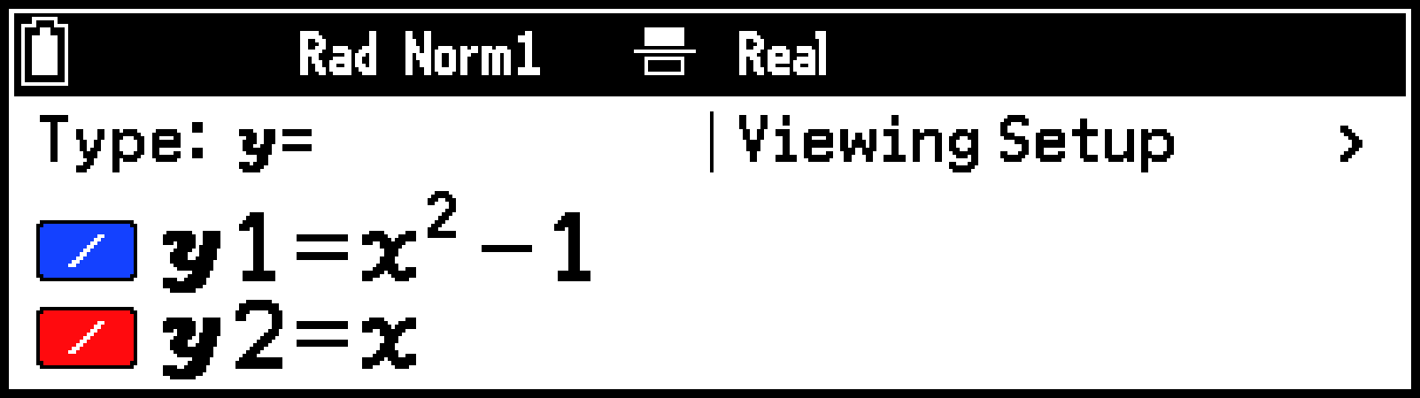
Example: To input the functions and , draw a graph, and create a numeric table
-
h > Graph&Table
-
On the Function tab, input the function.
-
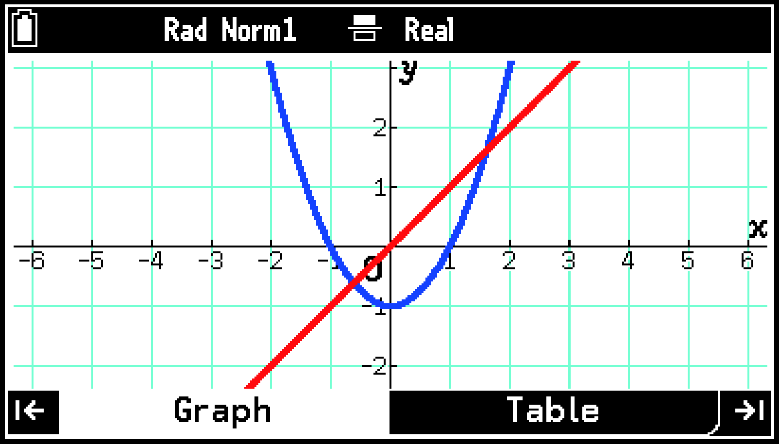
To draw a graph of the function you entered, press >.
-
Highlight
 and then press O.
 -
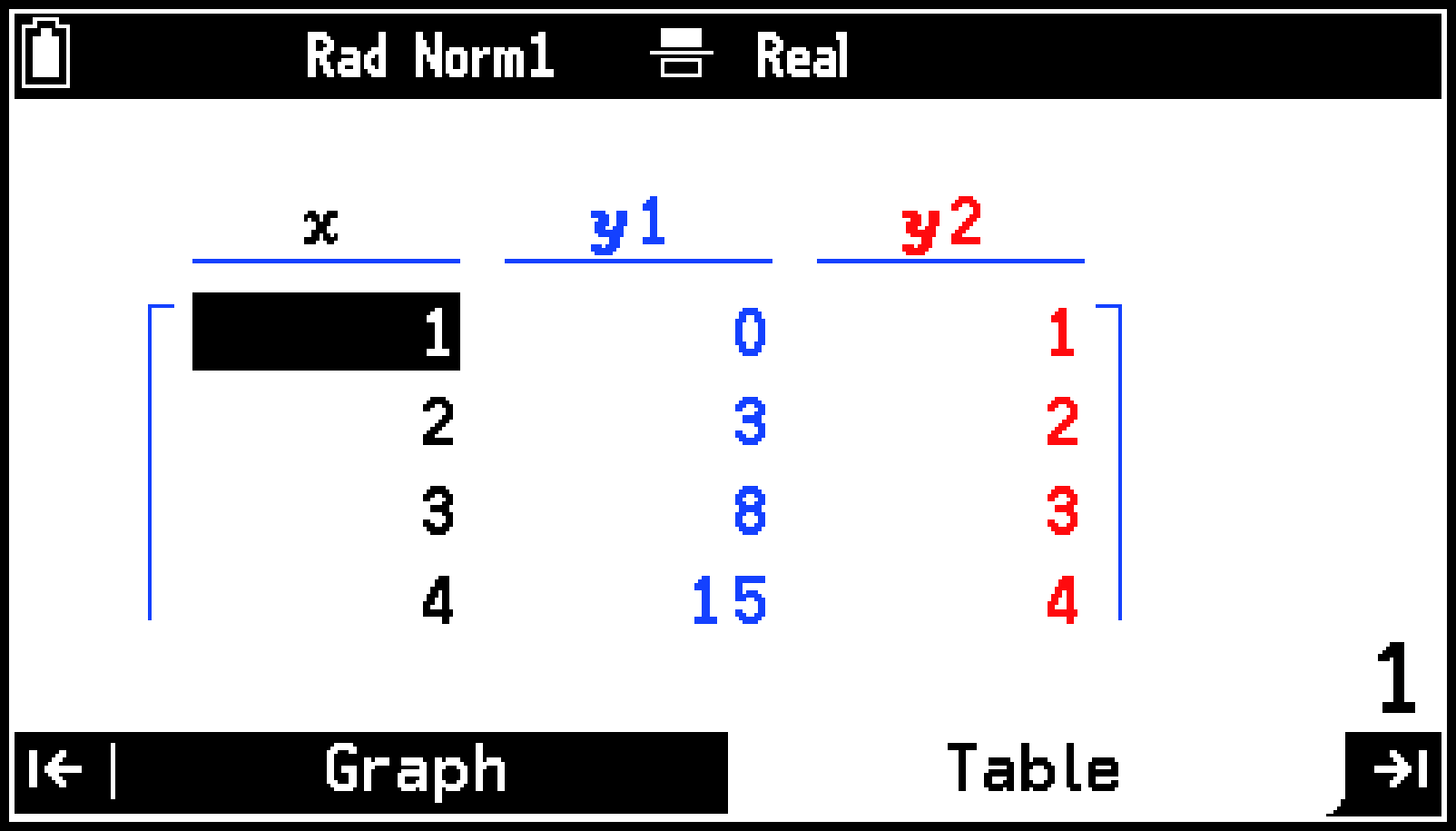
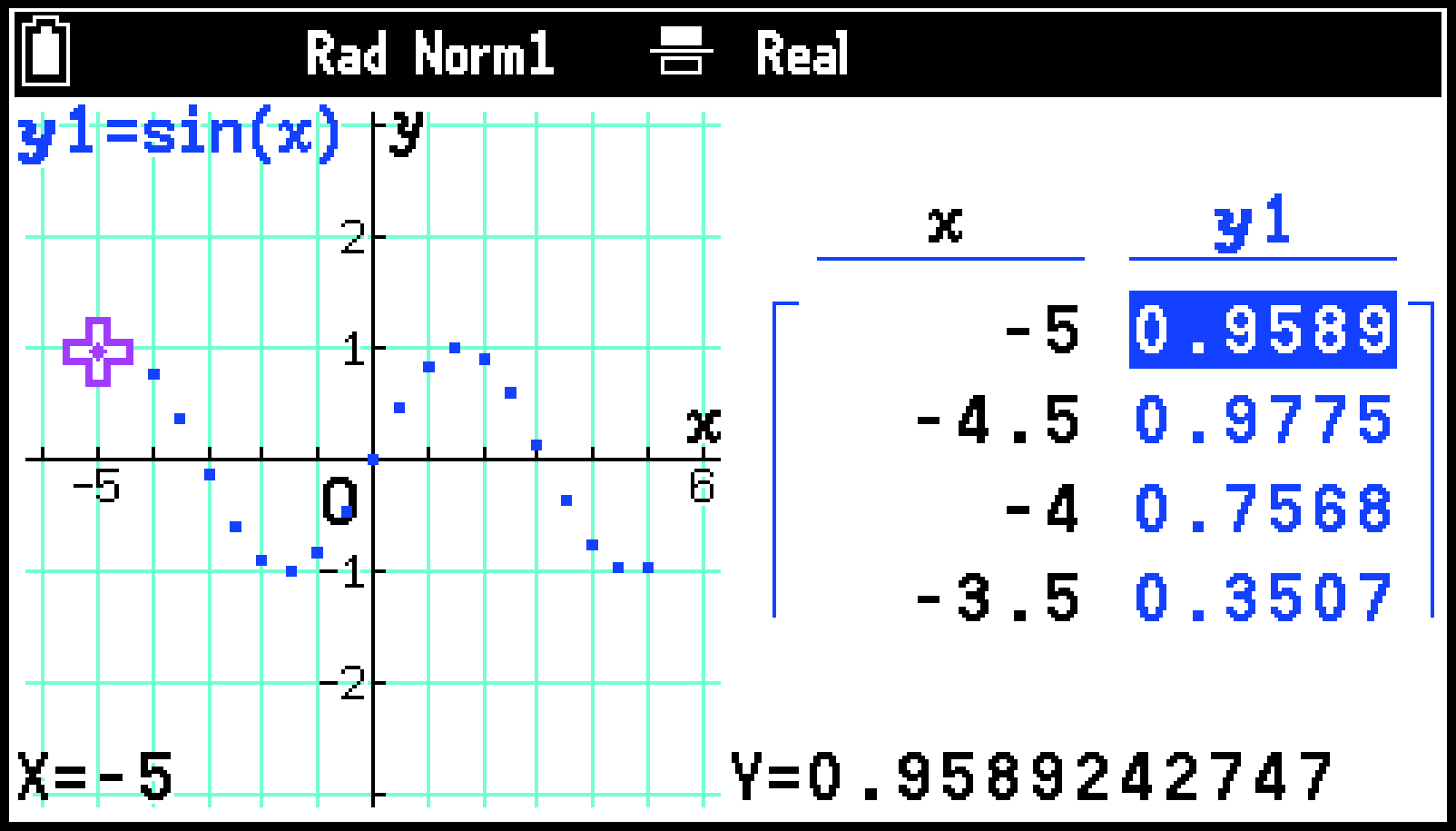
To display the numeric table for the function you entered, press >.
-
To return to the Function tab, press > or b.
(1) In the line, input .
(2) In the line, input .
Xi-1E
XE
This displays the View Window menu. Change the range specification as required. For more information, see Specifying the Display Range of the Graph Window (View Window).
This draws the graph on the Graph tab.
This displays the numeric table on the Table tab.
Note
Functions input on the Function tab of the Graph&Table app also appear on the Function tab of the Dyna Graph app. Similarly, functions input on the Function tab of the Dyna Graph app also appear on the Function tab of the Graph&Table app.
Out of Drawing Range Graph Warning Message
The Out of Drawing Range warning message appears when there is nothing to draw in the window when you try to draw a graph. If this happens, choose the desired operation from the menu that appears.
|
To do this: |
Select this menu item: |
|---|---|
|
Display the View Window menu |
[View Window] |
|
Automatically adjust View Window settings and draw a graph |
[Auto Zoom] |
|
Display the graph window (without drawing a graph) without adjusting View Window settings |
[Cancel] |
Using the Function Tab
Within the Function tab, you can enter up to 20 functions of various types.
Using the Setup Menu
Use the Setup menu to select a function type. You can also use this menu to specify the range of the graph window and numeric table.
To display the Setup menu
-
On the Function tab, highlight the first line.
-
Press O.
Pressing U always highlights the first line.
To select a function type
-
From the Setup menu, select [Type].
-
Perform the operations described in the table below.
This displays the Type menu.
|
To select this function type: |
Select this menu item: |
|---|---|
|
Cartesian coordinate type ( form) |
[=] |
|
Polar coordinate type ( form) |
[r=] |
|
Parametric type ( form) |
[Param] |
|
Cartesian coordinate type ( form) |
[X=] |
|
Inequality type (>, <, ≥, ≤ form) |
[>], [<], [≥], [≤] |
|
Inequality type (>, <, ≥, ≤ form) |
[X>], [X<], [X≥], [X≤] |
The type you choose is applied to the function you are about to input. It does not affect any function that has already been entered.
To specify the display range of the graph window
From the Setup menu, select [View Window]. See Specifying the Display Range of the Graph Window (View Window) for details.
To specify the numeric table domain
From the Setup menu, select [Set Table Domain]. See Specifying a Table Domain for details.
Inputting and Editing Functions
To input a function
-
Use the operation under To select a function type to select the type of function you want to input.
-
On the Function tab, highlight the line where you want to input, and then input a function.
Press X to input the variables (, , , ) according to the function type you chose.
Example 1: To input the form of Cartesian coordinate type
2Xi-2E
Example 2: To input the polar coordinate type
vX)-1E

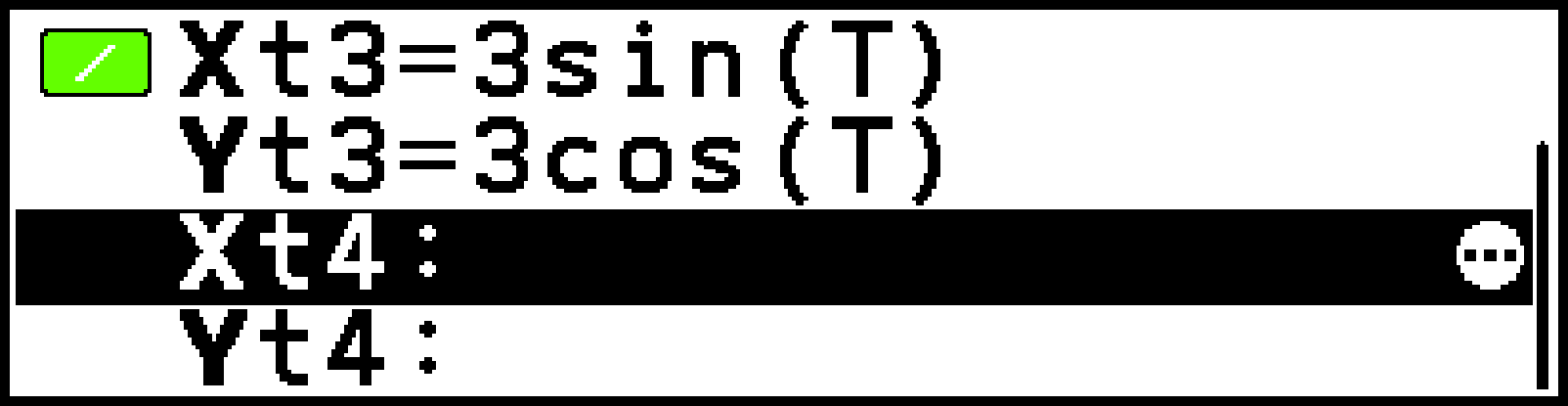
Example 3: To input parametric type
3vX)E
3cX)E
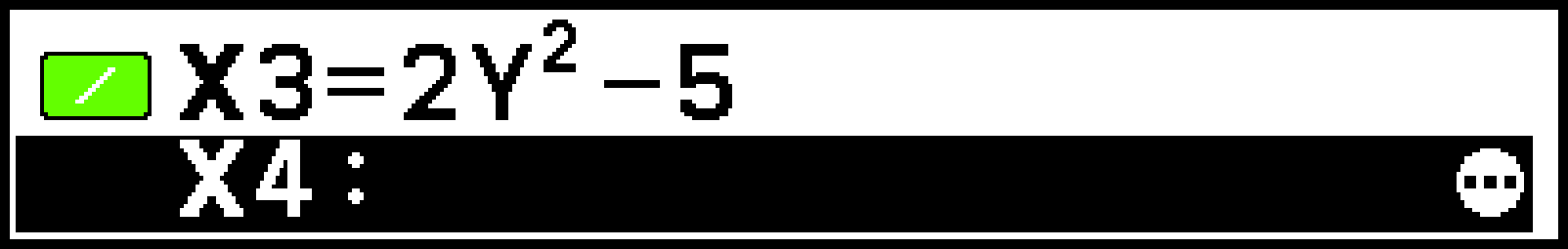
Example 4: To input the form of Cartesian coordinate type
2Xi-5E
In addition to the above, you can also use the special format input methods described below.
|
To do this: |
Perform this operation: |
|---|---|
Input a composite functionExample: To input the composite function “” into after and have already been input*1 |
Input “” into the line. V > [Function] > [1]( |
Input a function containing one or more alpha variable*2 while simultaneously specifying the value to be assigned to one of the alpha variables in the function*3*4Example: Assign 1, 2, 3 to variable of *5 |
Input “” into a line.*6*7 PX(A)Xi-1` |
Input a function that includes a list*3*4Example: Input *8 |
Input “” into a line. C > [Statistics] > [{ }] 1 ` 2 ` 3rXiE |
Input a function with a range of variable valuesExample: Specify the value of within the range 0 ≤ ≤ 2 |
Input “” into a line. Xi`s4([)0`2s5(])E |
Composite functions can be nested up to five levels.
Alpha variables except , , and .
If there are multiple variables or multiple elements in the list, multiple graphs will be drawn at the same time based on a single input function.
The color and line type of the graph drawn by this operation cannot be changed.
If there is only one value to be assigned, it can also be entered using the syntax ().
Be sure to input numeric values within the square brackets ([ ]). You cannot input alpha variables here.
Even if there are multiple variables in a function, values can be assigned to only one of the variables.
When multiple lists are used in a function, all of the lists must have the same number of elements. For example, . If a list does not have the same number of elements as the other lists, a Dimension ERROR will occur.
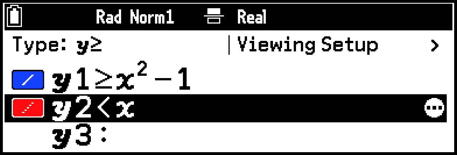
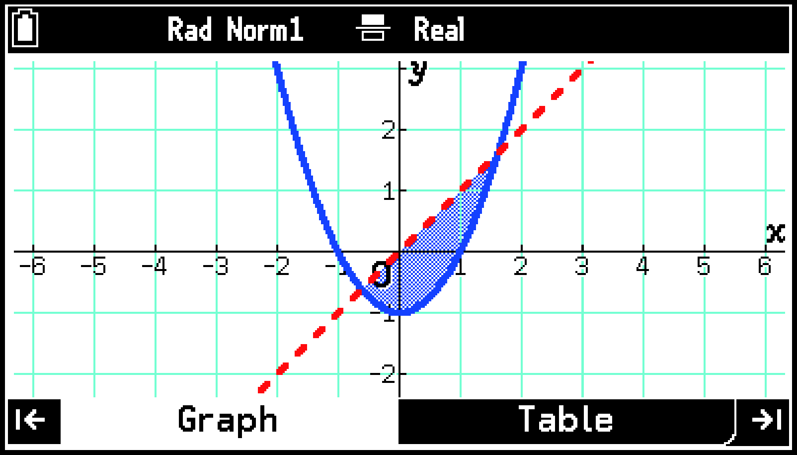
Inputting Inequalities and Configuring Fill Settings
Example: To input the inequalities ≥ and <
-
Use the procedure under To select a function type to select [Type] > [≥].
-
Input into the line and into the line.
-
Highlight the line and then select T > [Change Symbol] > [<].
-
Press > to draw the graph.
By default (S > [Ineq Region Type] > [Union]), all ranges satisfying the conditions of each inequality are filled.
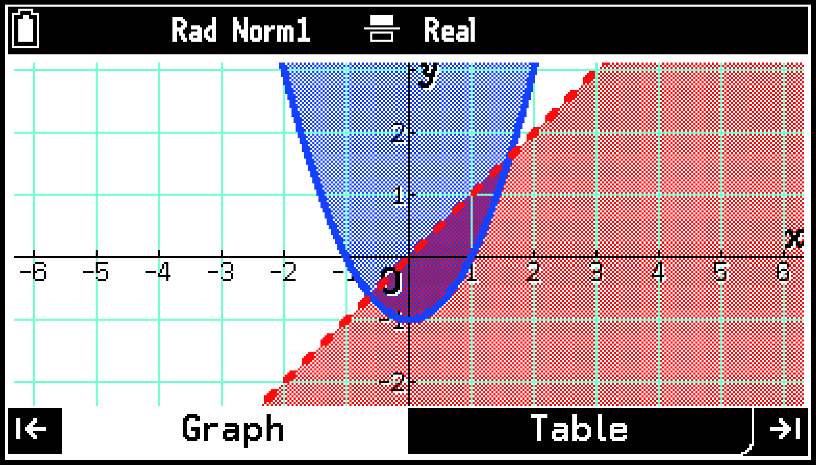
If you choose S > [Ineq Region Type] > [Intersection] to draw the graph, only the range that satisfies the conditions of all inequalities is filled.
To edit a function
On the Function tab, highlight the line you want to edit and then perform the operation below.
|
To do this: |
Perform this operation: |
|---|---|
|
Edit what you have already entered |
Press l, r, or E. This causes the input cursor to appear so you can edit the entry.* |
|
Overwrite input |
Press the key of the number or letter you want to re-input.* |
|
Change the symbol of a Cartesian coordinate type or inequality type |
T > [Change Symbol] and select a sign from the list displayed. |
Edits are not finalized until you press E after editing. To cancel editing without changing anything, press b before pressing E.
To delete a function
|
To do this: |
Perform this operation: |
|---|---|
|
Delete the function in the highlighted row |
Highlight the line that contains the content you want to delete,* and then press I. Or you could select T > [Delete] > [Delete Formula]. |
|
Delete all functions on the Function tab |
Press a. Or you could select T > [Delete] > [Delete All]. |
For parametric type functions, highlight either the or line.
Graph Drawing Settings (Line Type, Line Color)
On the Function tab, highlight the row that contains the graph drawing settings you want to change and then perform the operations described in the table below.
|
To do this: |
Perform this operation: |
|---|---|
|
Change the line type for graph drawing |
Select T > [Line Style]. Use the list that appears to select a line style. |
|
Change the line color for graph drawing |
Select T > [Line Color]. Use the list that appears to select a color. |
The line type and color you specify are shown by the icons to the left of each line of the Function tab.
Drawing Graphs and Creating Tables
To select a function to draw a graph and create a numeric table
-
On the Function tab, highlight a line that contains an input function.
-
Press T.
-
Change [Select] to
 (On) to enable or to
  (Off) to disable graphing and numeric table generation for the selected function.
 -
Press b to close the Tools menu.
This displays a Tools menu with [Select] highlighted.
The on/off setting of step 3 is indicated by the icons to the left of each line of the Function tab.
|
|
|
Note
All functions that you enable (turn on) in step 3 can be graphed, regardless of their type.
A numeric table can be created for a function that you enable (turn on) in step 3 if its function type selected for [Type] on the Setup menu is [=], [r=], or [Param].
To go from the Function tab to the Graph tab (to draw a graph)
Press > or highlight ![]() and then press O. This causes the View Window menu to appear so you can specify the range of the graph window. Change the range specification as required. For more information, see Specifying the Display Range of the Graph Window (View Window).
and then press O. This causes the View Window menu to appear so you can specify the range of the graph window. Change the range specification as required. For more information, see Specifying the Display Range of the Graph Window (View Window).
To return to the Function tab, press < or b.
Note
To prevent the View Window menu from appearing when you go to the Graph tab, turn off S > [Show V-Win Settings].
To go from the Function tab to the Table tab (to create a numeric table)
Press < or highlight ![]() and then press O.
and then press O.
To return to the Function tab, press > or b.
Note
If you want to add a column of derivative coefficients to the numeric table on the Table tab, turn on S > [Derivative]. In addition to the and columns, a ’-column for the derivative coefficient will be included in the numeric table.
Using the Graph Tab
Showing and Hiding Tabs
While the Graph tab is active, press D* to hide the tab and expand the graph window. Press U to show the tab again.


![]() in the lower-right corner of the window and
in the lower-right corner of the window and ![]() in the status bar indicate that a hidden tab can be shown again.
in the status bar indicate that a hidden tab can be shown again.
You can hide the tab by pressing O, a, or almost any other key. Tabs also may be hidden automatically when certain functions (such as graph analysis) are executed. ![]() is not displayed, the tab cannot be redisplayed until execution of the current function is stopped.
is not displayed, the tab cannot be redisplayed until execution of the current function is stopped.
Adjusting the Graph Window
To move the graph window up, down, left, or right
Use the cursor keys.
To zoom the graph window in or out
Press + to zoom in or - to zoom out.
To fine-tune the graph window (Tools menu)
|
To do this: |
Select this menu item: |
Details: |
|---|---|---|
|
Specify the display range |
T > [View Window] |
Specifying the Display Range of the Graph Window (View Window) |
|
Zoom the graph window in or out |
T > [Zoom] |
|
|
Grab a point on a window and drag it around the display |
T > [Pan] |
Grabbing a Point on a Window and Drag It Around the Display (Pan) |
|
Adjust the background image |
T > [Fade I/O] |
Specifying the Display Range of the Graph Window (View Window)
Use the View Window menu* to specify the display range (- and -axis range) of the graph window. You can also use this menu to specify the range of values for drawing polar and parametric type graphs.
This menu appears on the Graph tab when you select T > [View Window]. It can also be displayed from other tabs in the Graph&Table app, Dyna Graph app and the Recursion app. The menu contents are the same regardless of where it is displayed.
Using the Preset View Window Settings
|
To use this setting: |
Select T > [View Window] > [Pre-set Windows] and then select this: |
|---|---|
|
Initial calculator setup |
[Initialize] |
|
Presets according to the current angle unit setting (S > [Angle]) |
[Trigonometric] |
|
Calculator standard setup |
[Standard] |
|
Fix the current -axis setting and change the -axis setting so the on-screen -axis and -axis scale widths are one-to-one |
[Square] > [Y Base] |
|
Fix the current -axis setting and change the -axis setting so the on-screen -axis and -axis scale widths are one-to-one |
[Square] > [X Base] |
To specify the display range manually
Use the View Window to input values for the items below.
Minimum, Maximum, Scale (-axis minimum value, maximum value, scale)
Minimum*, Maximum, Scale (-axis minimum value, maximum value, scale)
Dot Value is the value per dot in the -axis direction. It is determined according to the values of Minimum and Maximum. Changing the Dot Value value automatically updates the Maximum value.
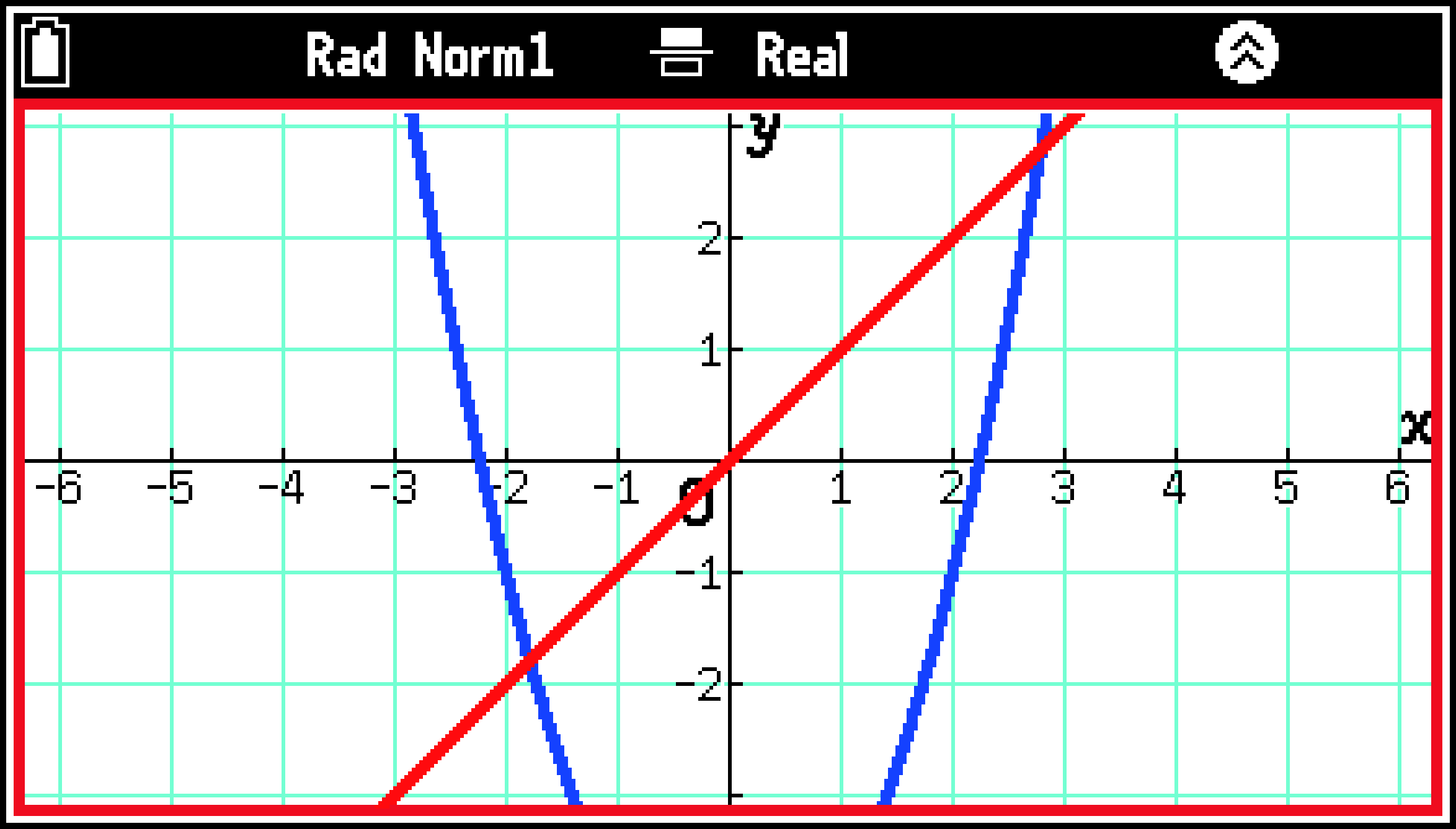
When the tab is hidden, the value set by Minimum is the bottom edge of the graph window (red frame below).
To specify the range of T and values and the pitch
These settings are applied when drawing parametric and polar graphs. Use the View Window to input values for the items below.
T,θ Minimum, T,θ Maximum (maximum and minimum values assigned to T in the parametric type function, and maximum and minimum values to be assigned to in the polar coordinate type function)
T,θ Pitch is the pitch of the T and values when drawing the graph. The smaller the pitch values, the finer the graph that is drawn. Larger values result in coarser graphs.
Changing the Graph Window Zoom Setting (Zoom)
Your calculator provides various convenient zoom settings that you can use to change the display range of the graph window.
|
To do this within the graph window: |
Select T> [Zoom] and then select this: |
|---|---|
|
Adjust the display so the graph is drawn along the entire -axis |
[Zoom Auto] |
|
Enclose a portion of the window and then zoom in on it |
[Zoom Box]*1 |
|
Zoom in or out on the center of the window*2 |
[Zoom In] |
|
Correct the -axis so the - and -axis scales are in a 1:1 ratio |
[Zoom Square] |
|
Make the displayed -coordinate value an integer when using trace |
[Zoom Integer]*3 |
|
Round the displayed -coordinate value to the appropriate number of significant digits when using trace |
[Zoom Round] |
|
Restore previous View Window settings for all subsequent zoom operations |
[Zoom Original] |
|
Reset to View Window settings in effect immediately before the last zoom operation |
[Zoom Previous] |
Selecting T > [Zoom] > [Zoom Box] displays a cross pointer (![]() ) in the window. Move the pointer to one of the box’s vertices and then press O. Next, move the pointer to the opposite vertex and then press O.
) in the window. Move the pointer to one of the box’s vertices and then press O. Next, move the pointer to the opposite vertex and then press O.
The zoom in/out ratio is the one specified in the dialog that appears when you select T > [Zoom] > [Zoom In/Out Factors].
Selecting T > [Zoom] > [Zoom Integer] displays a pointer in the window. Move the pointer to the coordinate you want to center in the window and press O.
Grabbing a Point on a Window and Drag It Around the Display (Pan)
You can use the hand icon that appears to drag the graph window around the display.
-
While the graph window is displayed, select T > [Pan].
-
Use the cursor keys to move the arrow pointer to the point in the window that you want to grab and then press O.
-
Use the cursor keys to move the hand and drag the window around the display.
-
Press O.
This displays an arrow pointer (![]() ).
).
This causes the pointer to change from an arrow (![]() ) to a hand (
) to a hand (![]() ).
).
The contents of the window move along with the hand.
This returns the pointer to an arrow. You can repeat steps 2 and 3 as required.
When you are finished dragging window contents, press b.
Adjusting the Graph Window Background Image (Fade I/O)
You can use this operation to adjust the opacity of the background image. This operation can be performed only when a 16-bit color image is being used as the graph window background image. For information about displaying a background image, see Background (Graph).
-
While the graph window is displayed, select T > [Fade I/O].
-
Use l and r to adjust the opacity of the background image.
-
When the setting is the way you want, press b.
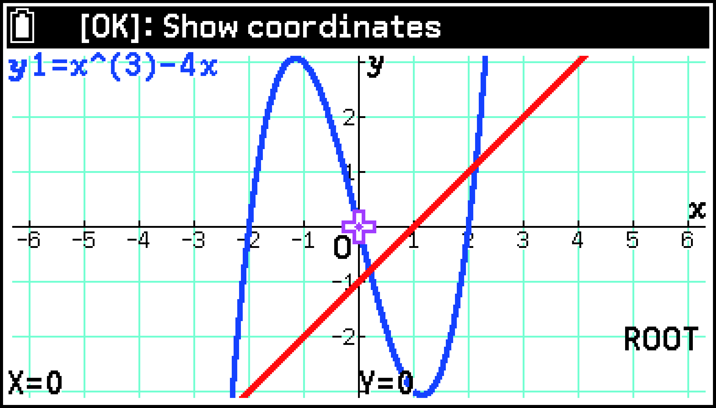
Using Graph Solve (Graph Solve)
You can use Graph Solve to obtain the coordinates of roots, and other values for the integrals, -axis intercept, or other key feature points on a graph. For example, perform the operation below to find the root of a function on a graph.
-
Enter the function in the Function tab and press > to draw a graph.
-
Select T > [Graph Solve] > [Root].
-
Use d and u to move the flashing to the graph whose root you want to obtain and then press O.
-
To exit graph analysis, press b.
If there are multiple graphs in the graph window, one of them will flash.
This causes a cross pointer (![]() ) to appear at the coordinates of the root and the coordinate values to appear at the bottom of the window. If there are multiple roots, you can use r and l to move the pointer to another root.
) to appear at the coordinates of the root and the coordinate values to appear at the bottom of the window. If there are multiple roots, you can use r and l to move the pointer to another root.
The values that can be obtained using graph analysis are shown in the table below.
|
To obtain this value: |
Select T > [Graph Solve] and then select this: |
|---|---|
|
Roots on a graph |
[Root] |
|
Maximum value on a graph |
[Maximum Value] |
|
Minimum value on a graph |
[Minimum Value] |
|
Coordinates of intersection of two graphs*1 |
[Intersection] |
|
Integral value of the specified range on the graph*2 |
[] > [] |
|
Integral value and area*2*3 of a range delimited by multiple roots on the graph |
[] > [Root] |
|
Integral and area*2*4 of a range bounded by multiple intersections of two graphs |
[] > [Intersection] |
|
Integral and area*2*5 of a range bounded by the intersection of two graphs and a root on either of them |
[] > [Mixed] |
|
-axis intercept |
[y-Intercept] |
|
-coordinate value on a graph for a given -value*6 |
[x-Cal] |
|
-coordinate value on a graph for a given -value |
[y-Cal] |
Can be calculated for Cartesian coordinate type ( form) and inequality type (>, <, ≥, ≤ form) graphs.
Can be calculated for Cartesian coordinate type ( form) graphs.
An error occurs if there are more than 21 roots between the two specified roots.
An error occurs if there are more than 21 intersections between the two specified intersections.
You can also use the number keys to specify any -coordinate value instead of the intersections or roots of the graph.
Cannot be calculated for parametric type graphs.
Important!
In the cases described below, solution accuracy may be reduced or solution may be impossible.
When the solution is at the point of tangency between graphs or at the point of tangency between a graph and the -axis.
When the solution is at or near the inflection point of a graph.
Operation Example:
Example 1: To graph and , specify two intersections, and then calculate the integral and area between them
-
Graph the two functions.
-
Select T > [Graph Solve] > [] > [Intersection].
-
Press O to make the current pointer location the lower limit of integration.
-
Press r twice to move the pointer two intersections to the right.
-
Press O to make the current pointer location the upper limit of integration.
-
To exit graph analysis, press b.
This causes a pointer to appear at the coordinate of the leftmost intersection.
This defines the integral range and displays the calculation result.
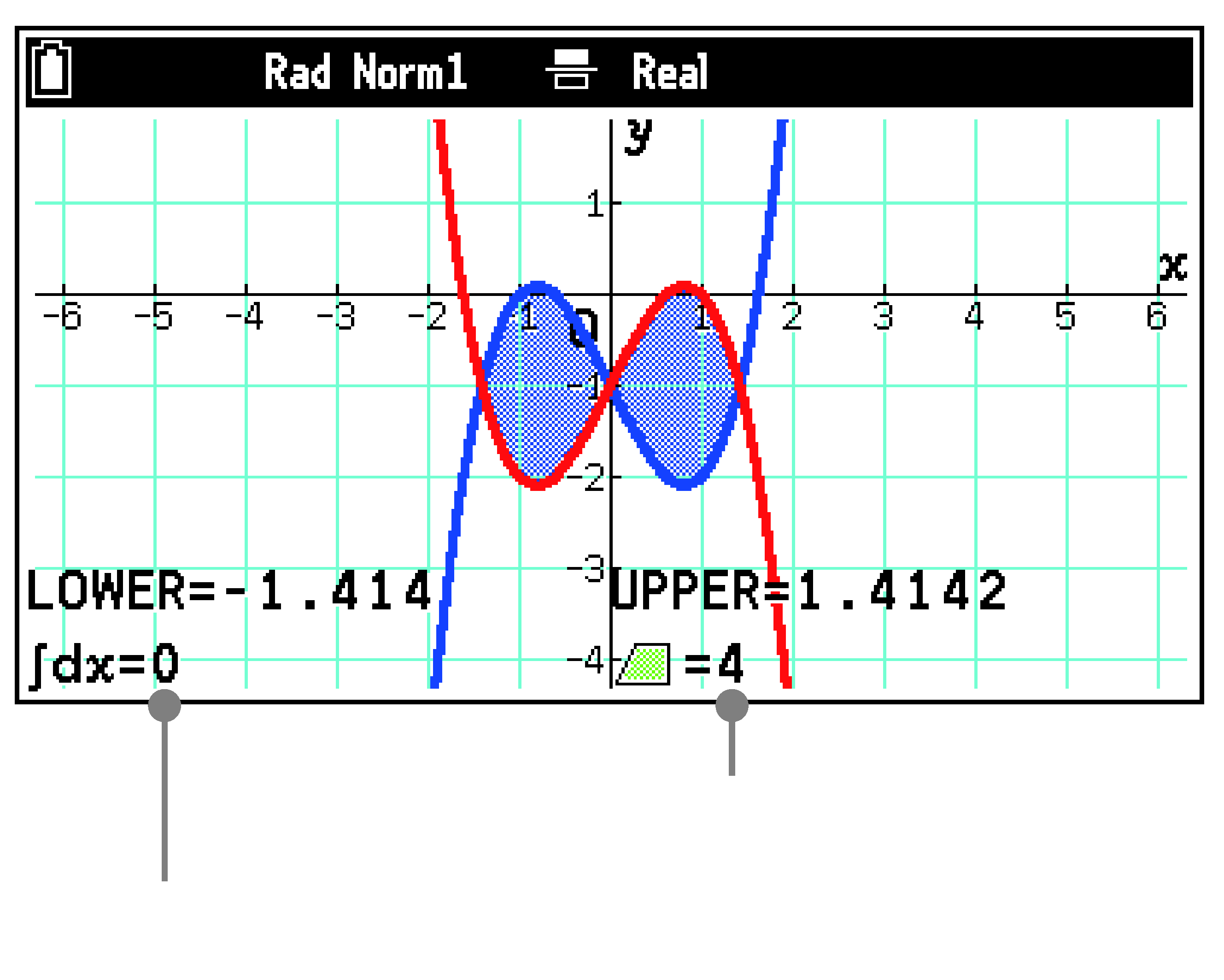
Integral value
Area
Example 2: To calculate the -value of the graph you drew in Example 1 above when -0.5
-
Select T > [Graph Solve] > [x-Cal].
-
Use d and u to move the flashing to the graph of and then press O.
-
Input -0.5 and then press O.
-
To exit graph analysis, press b.
This displays a dialog for inputting the -value.
This will cause a pointer to appear at one of the coordinates where -0.5 and the coordinate value will appear at the bottom of the window. You can use r and l to move the pointer to another coordinate where -0.5.
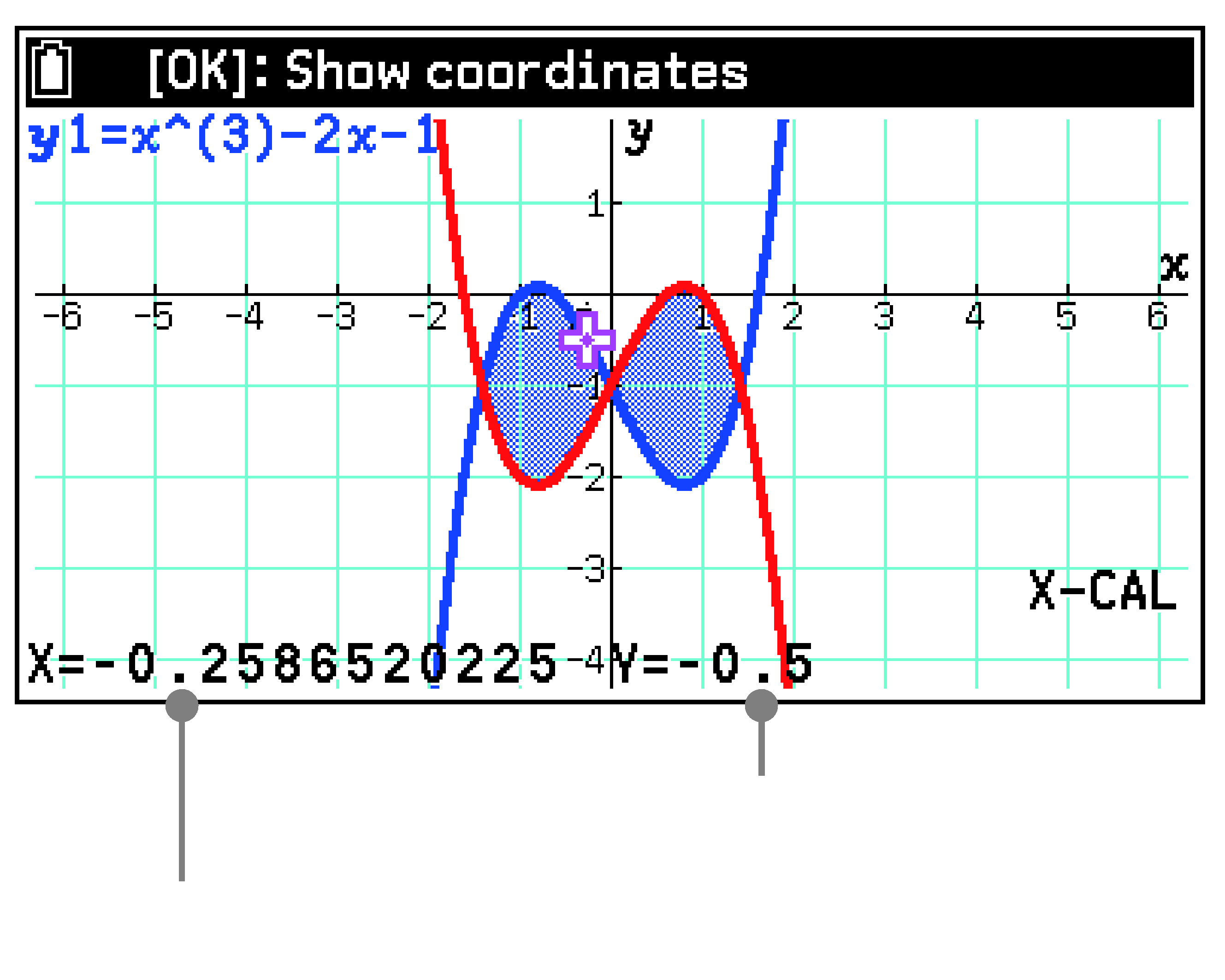
-coordinate value
-coordinate value
Using Trace (Trace)
Trace displays a crosshair pointer (![]() ) on a graph that you can use to read the coordinate values at a specific location. When S > [Derivative] is turned on, derivative coefficients are displayed along with the coordinate values.
) on a graph that you can use to read the coordinate values at a specific location. When S > [Derivative] is turned on, derivative coefficients are displayed along with the coordinate values.
To enable trace
Select T > [Trace].
The operations that can be performed while the trace function is enabled are described in the table below.
|
To do this: |
Perform this operation: |
|---|---|
|
Move the pointer along the graph |
Press l or r. |
|
Move to pointer to a specific -coordinate on the graph |
Use the number keys to input an -coordinate value and then press O. |
|
When there are multiple graphs, the pointer will move between them |
Press d or u. |
|
Plot a dot with coordinate values on a graph* 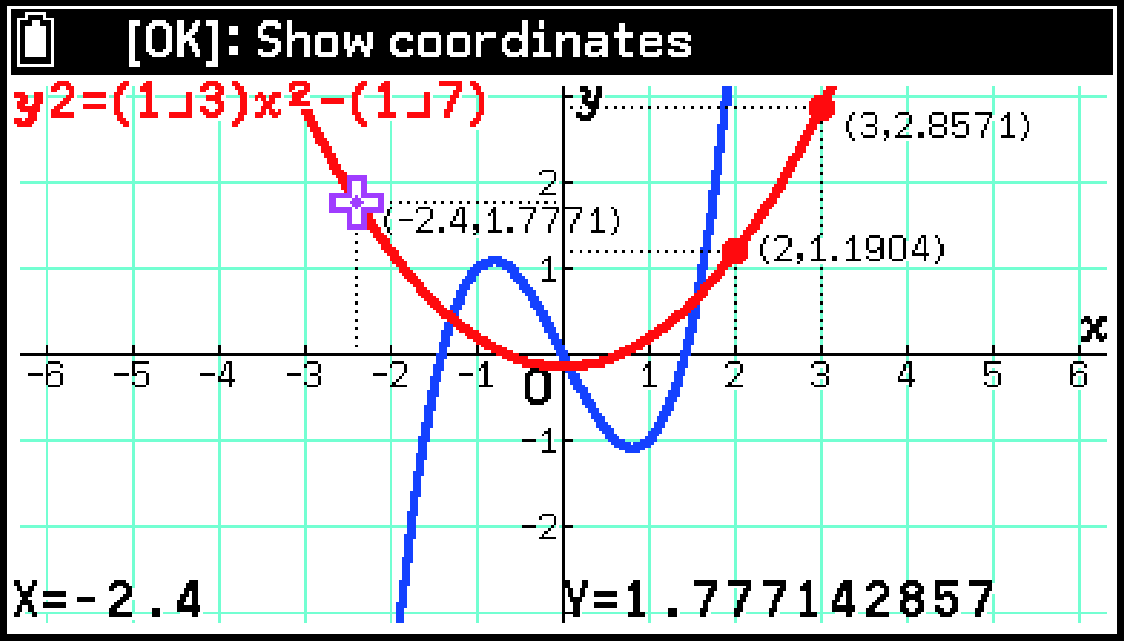 |
Move the pointer to the location where you want to plot a dot with coordinate values and then press O. |
|
Exit trace |
Press b. |
If the dot location is within the coordinates of a graph, it is displayed as a solid red dot (![]() ). If the dot location is not within the coordinates of the graph, it is displayed as a red circle (
). If the dot location is not within the coordinates of the graph, it is displayed as a red circle (![]() ).
).
Modifying a Graph by Changing the Coefficient Values of Its Function (Modify)
You can input a functional expression with five alpha variables included in the coefficients (such as ) and then change the values of the variables (coefficient values) while the graph is displayed. This lets you see how changes in the coefficient values affect the appearance of the graph.
Important!
When multiple functions are selected for graphing, modify cannot be used if there are more than two functions that contain variables.
Example: Input and observe how the shape of the graph is affected when the coefficient values are changed. The initial values of A, B, and C are , , and .*1
-
On the Function tab, input .
-
Turn off all other function expression graphing settings.
-
Press > to draw the graph.
-
Select T > [Modify] to enable modify.
-
Use l and r to change the value of A.
-
Press d to move the pointer (I) to B. Use l and r to change the value of B.
-
Press d to move the pointer (I) to C. Use l and r to change the value of C.
-
To exit modify, press b.
Select T > [Built-In Function] > [=A^2+B+C] and then input the function.*2
See To select a function to draw a graph and create a numeric table.
The current values of A, B, and C and the step value are displayed in the lower-left corner of the graph window. You can change the value where the pointer (I) is currently located.
Use d and u to move the pointer (I) up and down.
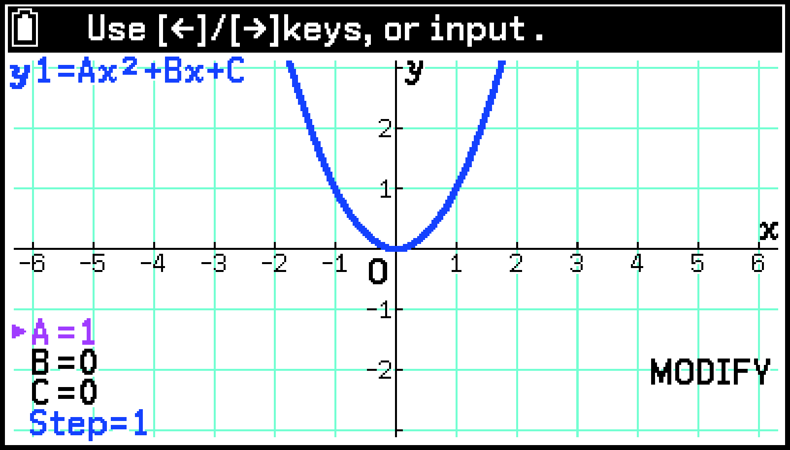
Each press of l or r changes the value of A by the step value. You can also use the number keys to enter values.
Assign , , and before beginning. See To assign a value to an alpha variable.
You can use T > [Built-In Function] to input the functions below.
Note
While modify is enabled, you can copy the function of the currently displayed graph to any function area on the Function tab (except an area of a function currently being used for drawing). To copy the function, select T > [Copy] and choose the destination area on the menu that appears.
Using Sketch (Sketch)
You can use sketch to draw dots, lines, and text within the graphing area. For example, to draw a tangent line on the graph of , perform the steps below.
-
On the Function tab, input the function and then press > to graph it.
-
Select T > [Sketch] > [Tangent Line].
-
To view the coordinates of the point of tangency, press O.
-
To exit sketch, press b.
This example graphs only.
This draws a line that is tangent to of the graph. You can use l or r to change the coordinates of the point of tangency.
This executed the tangent line drawing and displays a dot (![]() ) with coordinate values at the point of tangency.
) with coordinate values at the point of tangency.
Now you can use l and r to change the coordinates of the point of tangency and add a tangent line by pressing O.
The following table shows what you can do with sketch.
|
To do this: |
Select T > [Sketch] and then select this: |
|---|---|
|
Clear all points, lines, and text drawn using sketch |
[Clear Screen] |
|
Draw a line tangent to a graph |
[Tangent Line] |
|
Draw a graph normal line |
[Normal Line] |
|
Draw the inverse graph of a graph*1 |
[Inverse] |
|
Toggle a point between draw and delete |
[Plot] |
|
Specify two points and draw a line segment between them |
[Line] |
|
Draw a circle by specifying its center point and one point on the circumference |
[Circle] |
|
Draw a vertical line |
[Vertical Line] |
|
Draw a horizontal line |
[Horizontal Line] |
|
Draw a freehand line*2 |
[Pen] |
|
Write text*3 |
[Text] |
Sketch is automatically exited after a graph is drawn.
You can use the cursor keys to move the pointer and draw a line.
Input is possible starting from the current pointer location and ending with the right edge of the graph window. I key operations while input is in progress are ignored.
Note
Sketch points, lines, and text are drawn according to the settings of S > [Plot/Line Color] and S > [Sketch Line].
Graphing a Function Copied to the Clipboard
You can copy a function* from another app, paste it onto the Graph tab and then graph it.
An form expression (such as ) or a form equation (such as ).
Example: To copy , paste it onto the Graph tab, and then graph it
-
Use the Calculate app to input and then copy the expression.
-
Start up the Graph&Table app and then press > to graph the expression.
-
Press s.(%).
For details about the copy operation, see Copying, Cutting, and Pasting Expressions.
This graphs .
Graph Drawing Setting Items
You can use the Settings menu to configure settings for the graph drawing operation and the graph drawing display area. For details, see Settings Menu Details.
Using the Table Tab
With the Table tab, you can edit the numbers in the -column of a numeric table and also perform the operations below from the menu that appears when you press T.
|
To do this: |
Select this menu item: |
Details: |
|---|---|---|
|
Specify the domain of the table being created |
T > [Set Table Domain] |
|
|
Draw a graph that shows dots at the coordinates of a numeric table |
T > [Graph Points] |
|
|
Draw a graph that connects the coordinates of a numeric table with straight line segments |
T > [Graph Points (Joined)] |
|
|
Specify the display range of the graph window |
T > [View Window] |
Specifying the Display Range of the Graph Window (View Window) |
|
Insert or add a row |
T > [Row] |
|
|
Edit input data |
T > [Edit] |
|
|
Save one column of a numeric table to a list variable |
T > [Store List] |
|
|
Delete one row of a numeric table or the entire table |
T > [Delete] |
Specifying a Table Domain
The numeric table domain is specified by the value of the -variable (or , T) that is assigned to the function used to create the numeric table. The following two methods are available to specify a table domain.
|
To specify a table domain using this method: |
Perform this operation: |
|---|---|
|
Inputting the -variable starting value, ending value, and step value |
|
|
Using list variable elements as the -variable |
|
Graphing a Numeric Table
-
While the numeric table is displayed, select one of the options below.
-
Use the View Window menu that appears to change display range settings as required.
-
Highlight
and then press O.
To draw a graph of coordinate dots only: T > [Graph Points]
To draw a graph by linking coordinate dots with straight line segments: T > [Graph Points (Joined)]
For details, see Specifying the Display Range of the Graph Window (View Window).
This draws the graph on the Table tab.
Note
To prevent the View Window menu from appearing when drawing a graph, turn off S > [Show V-Win Settings].
The operations that can be performed while viewing a graph are the same as those on the Graph tab (except for [Graph Solve] and [Modify]).
Editing a Numeric Table
|
To do this: |
Perform this operation: |
|---|---|
|
Overwrite a numeric table -value* with a different value |
Move the cursor to the -column* line whose value you want to change and then input the new value. |
|
Edit a numeric table -value* |
Move the cursor to the -column* line you want to edit and then select T > [Edit]. |
|
Add one row below the row where the cursor is currently located |
Select T > [Row] > [Add]. |
|
Insert a row above the row where the cursor is currently located |
Select T > [Row] > [Insert]. |
|
Delete the row where the cursor is located |
Select T > [Delete] > [Row]. |
|
Delete the entire numeric table and return to the Function tab |
Select T > [Delete] > [Table]. |
, , or T
Saving a Numeric Table to a List Variable
One column of numeric table data can be saved to a list variable, which is specified by its number.
-
Move the cursor to the numeric table column you want to save to a list variable.
-
Select T > [Store List].
-
Use the dialog that appears to input a list variable number and then press O.
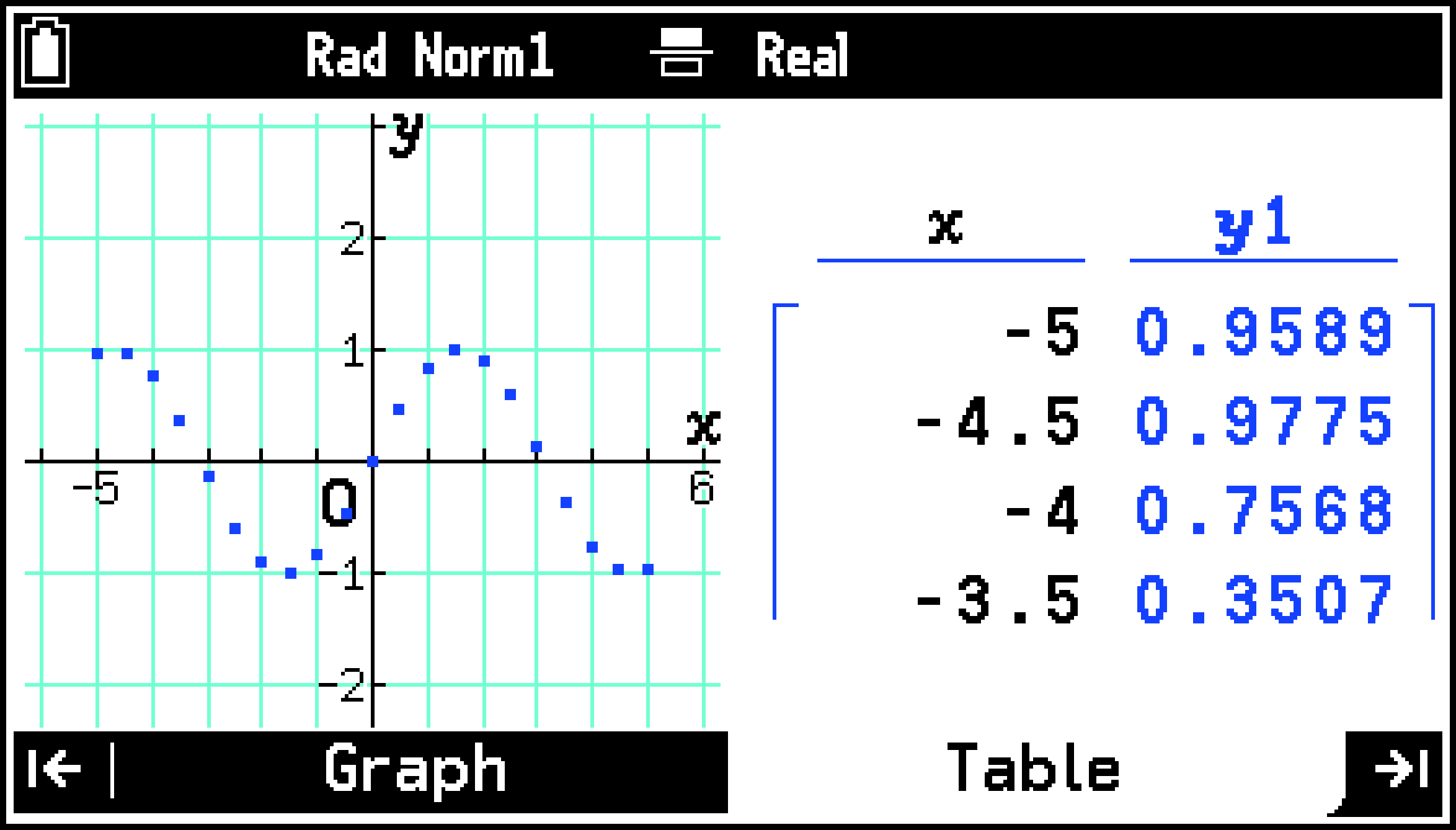
Displaying a Numeric Table and Graph at the Same Time
When S > [Table with Graph] is turned on, the numeric table window is displayed on the right of the Table tab, and the graph window is displayed on the left.
Nothing is drawn in the graph window immediately after you go from the Function tab or the Graph tab to the Table tab. Use the following operations to draw the graph.
Select T > [Switch Active Window].
From T, select [Graph Points] or [Graph Points (Joined)].
Each time you select T > [Switch Active Window], the active window (the window that is affected by the operations you perform) toggles between the numeric table window and the graph window. The numeric table window is active when the cursor is displayed on the numeric table.
The operations below can be used while the numeric table window is active.
You can perform the operations below while the graph window is active.
Adjusting the Graph Window (Excluding Pan and Fade I/O)
Specifying the Display Range of the Graph Window (View Window)
To display a pointer on a graph at the current numeric table cursor location (Graph-Link)
-
Turn on S > [Table with Graph].
-
On the Function tab, input the function and then press < to go to the Table tab.
-
Select T > [Switch Active Window].
-
Select T > [Graph-Link].
-
To exit this operation, press b.
This makes the graph window active and draws the graph.
This causes a crosshair pointer to appear on the graph at the coordinates that correspond to the numeric table cursor position.
Using d and u to move the numeric table cursor also causes the graph pointer to move accordingly.
Note
If no graph is drawn in the graph window, the T > [Graph-Link] cannot be performed while the numeric table window is active. T > [Graph-Link] becomes enabled after a graph is drawn in the graph window.