Financial App
You can use the Financial app to perform a variety of financial calculations.
Important!
Calculation results and graphs produced in this app should be regarded as reference values only.
Whenever performing an actual financial transaction, be sure to check any calculation results obtained using this calculator against the figures calculated by your financial institution.
Whether you should use a positive or a negative value for the present value (PV) or the purchase price (PRC) depends on the type of calculation you are trying to perform.
Operation Flow
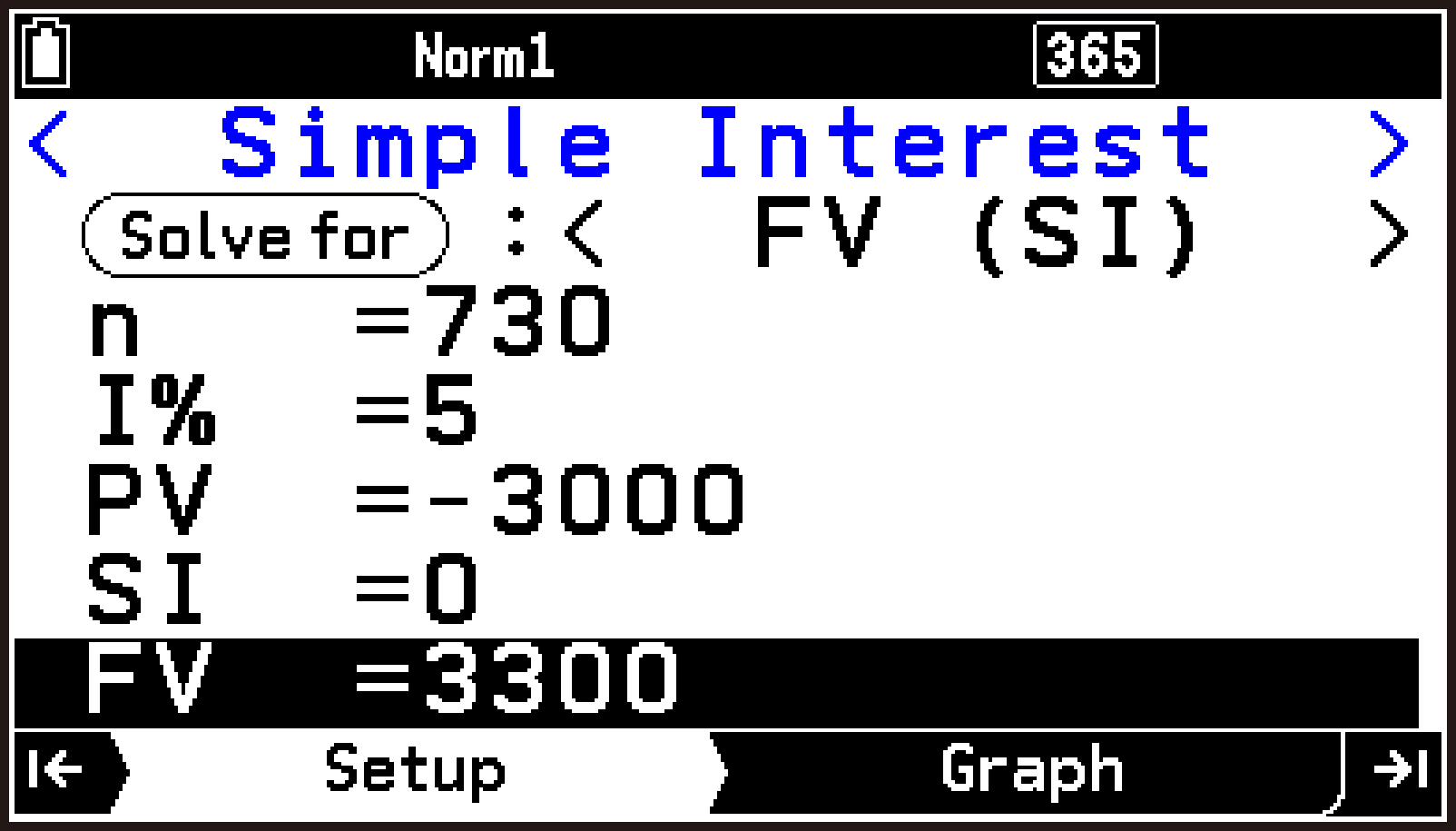
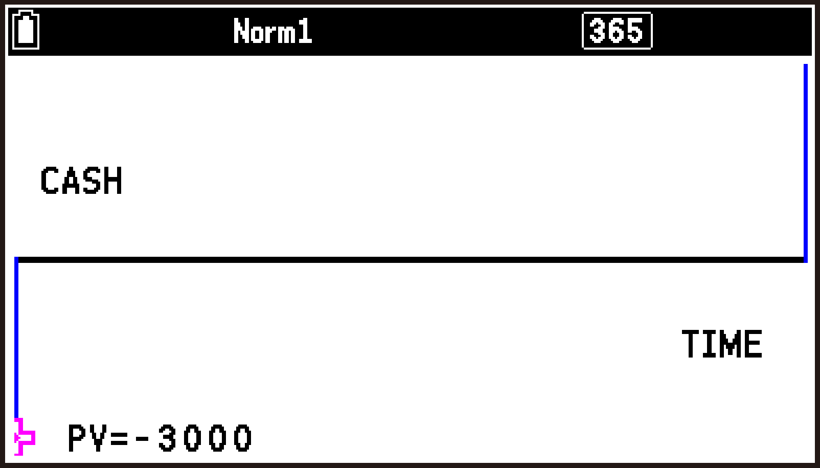
Example: To calculate the total principal and interest after two years (730 days*) when $3,000 is invested at a simple interest rate of 5.0%, and then to display a graph and check the calculation results against the graph
-
h > Financial
-
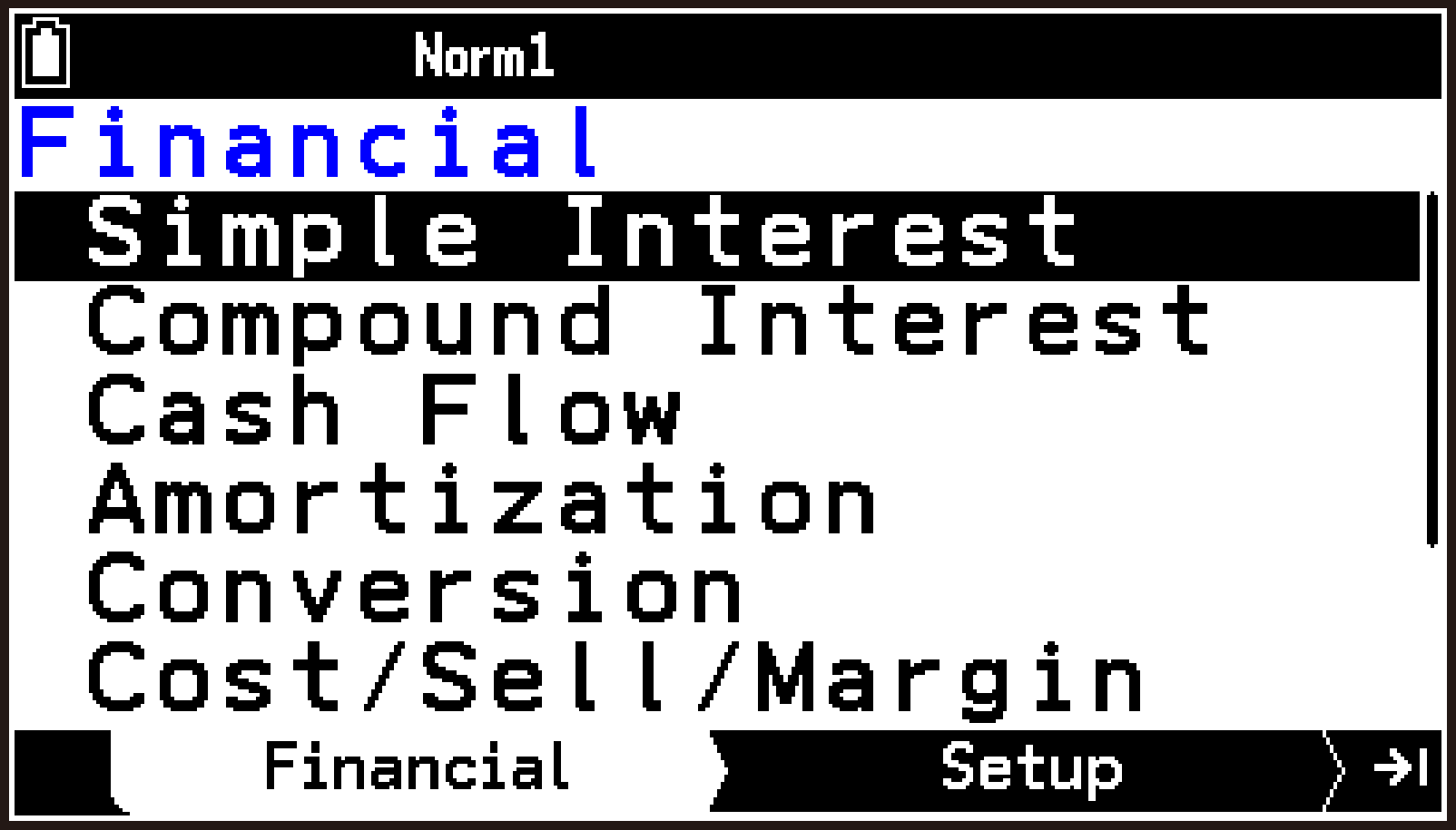
Highlight [Simple Interest] and then press O.
-
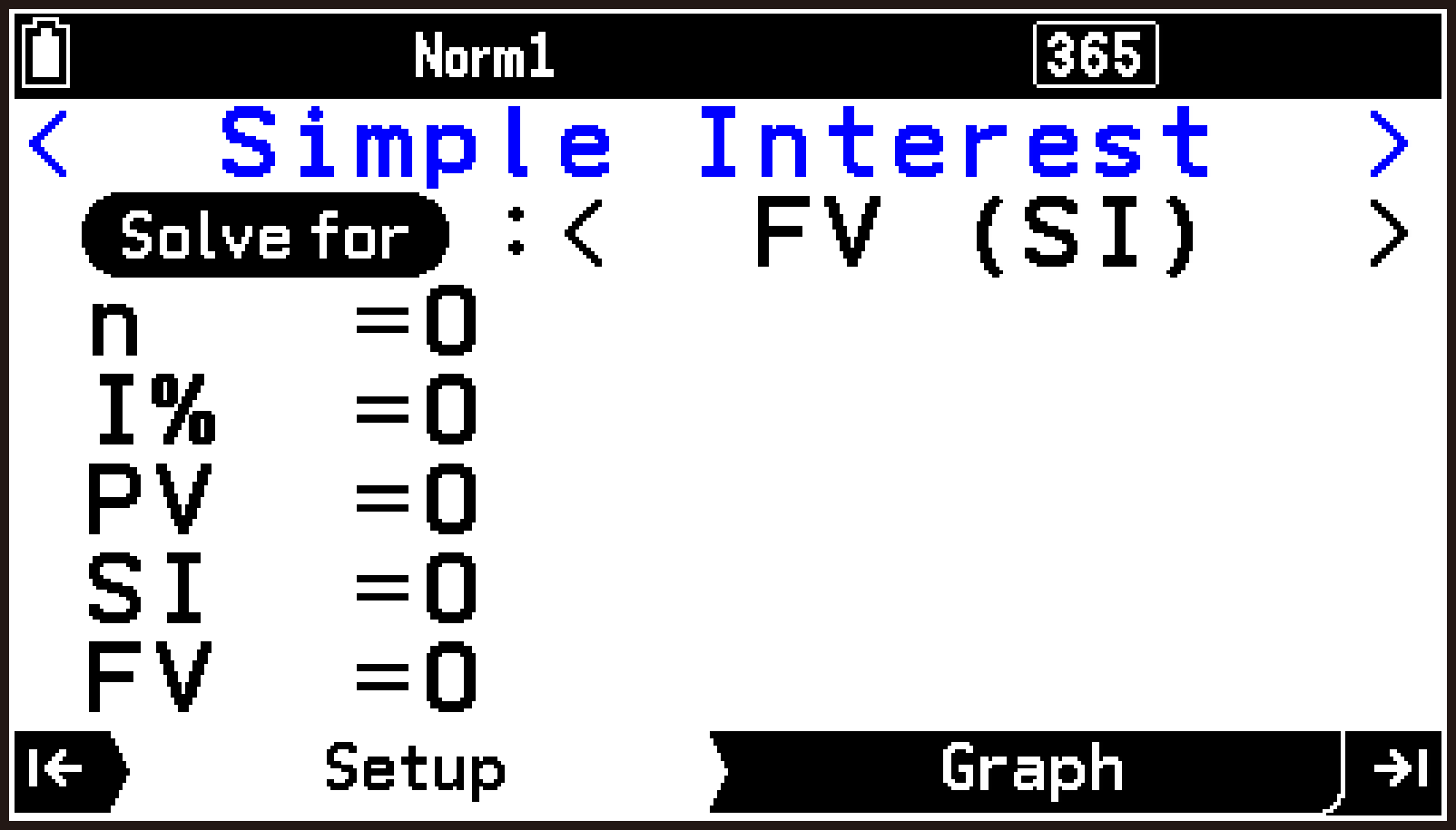
Select the item you want to calculate.
-
Press d to highlight the
 button.
 -
Use l or r to select the item you want to calculate.
-
Input the following information: n (days) = 730; I% (annual interest rate) = 5; PV (present value) = -3000.
-
Specify the color that you want to use for the graph in step 7 of this procedure.
-
Select T > [Graph Color].
-
Select the color you want and then press O.
-
To execute the calculation, press U to highlight
, and then press O. -
To display the graph, press >.
-
To check the calculation results on the graph, select T > [Trace].
-
To return from the Graph tab to the Setup tab, press b or <.
This displays the Financial tab.
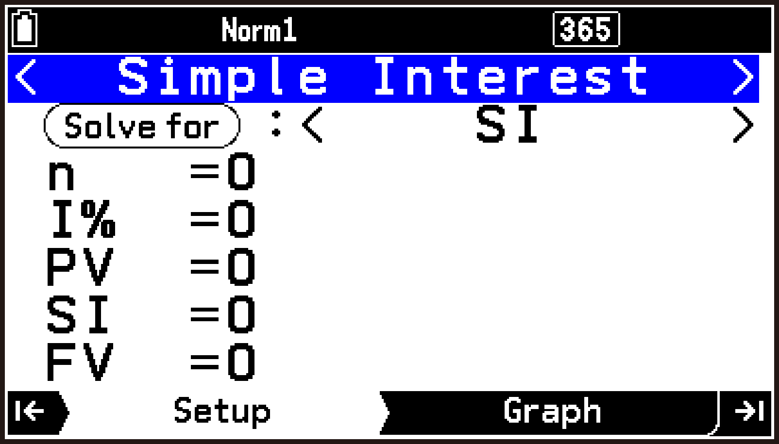
This displays the Simple Interest Setup tab.
|
To calculate this: |
Display this item: |
|---|---|
|
Simple Interest |
SI |
|
Future Value (SI) |
FV (SI) |
Since we want to calculate the future value, display “FV (SI)” here.
d730E5Es-(M)3000E
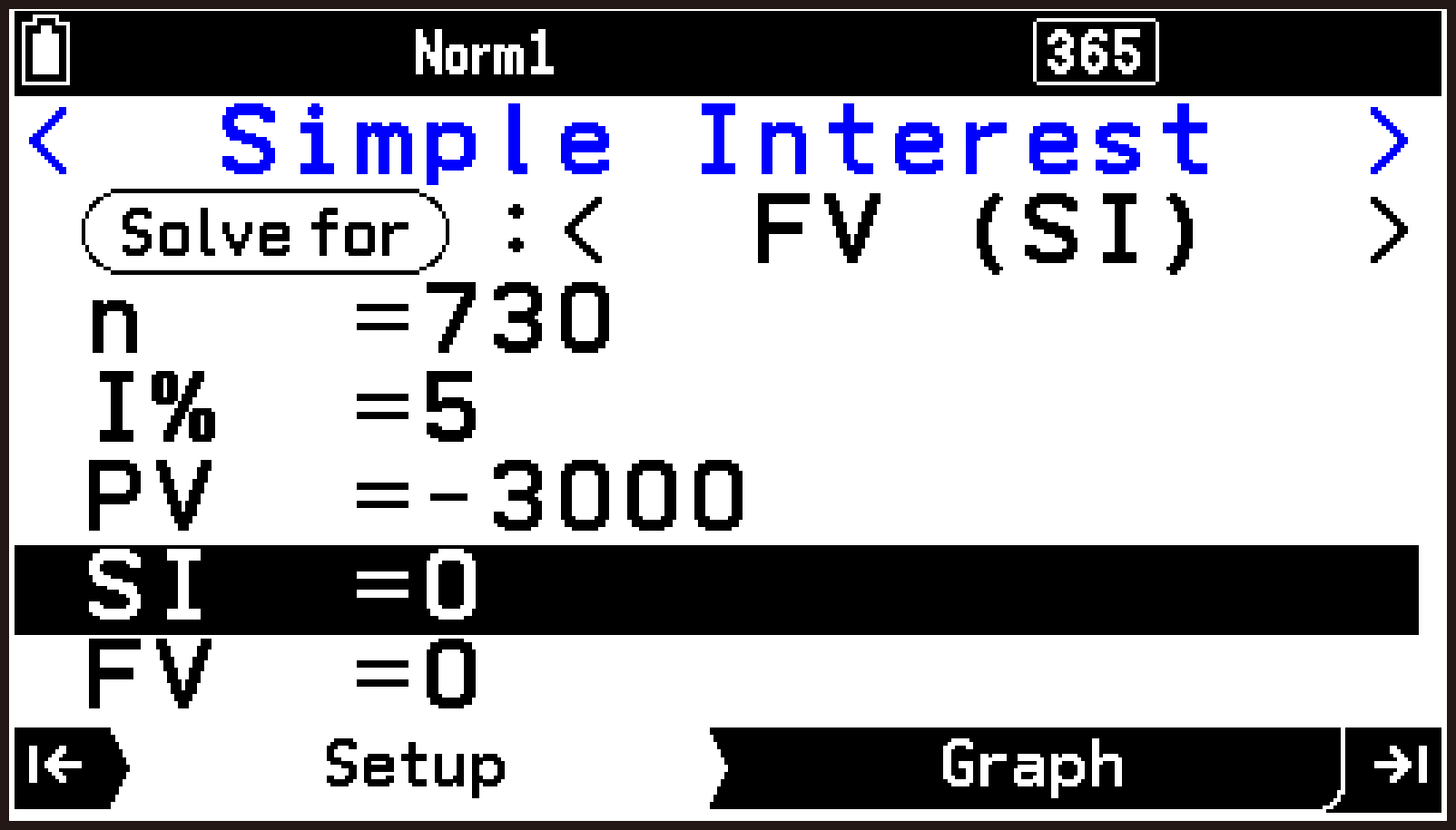
This moves the highlighting to the FV line and displays the calculation result for future value (FV = principal + interest).
An error occurs if parameters are not configured correctly.
This enables trace and causes a crosshair pointer ( ) to appear on the graph.
Each press of r while trace is enabled cycles the displayed value in the sequence: present value (PV) → simple interest (SI) → future value (FV). Pressing l cycles in the reverse direction.
To exit trace, press b.
Note
You can also use the procedure below instead of step 3 above.
-
Select T > [Solve for].
-
Use d or u to select [Future Value (SI)], and the press O.
The SI and FV lines are for displaying results only. You cannot input values in these lines.
Performing Financial Calculations
The calculations in the table below can be performed with the Financial app.
|
To perform this type of calculation: |
Select this for the financial calculation mode: |
|---|---|
|
Interest without compounding based on the number of days money is invested |
Simple Interest*1 |
|
Interest based on compounding parameters specified by you |
Compound Interest*2 |
|
Value of money paid out or received in varying amounts over time |
Cash Flow |
|
Interest and principal portions of a payment or payments |
Amortization*2 |
|
Effective or nominal interest rate for interest compounded multiple times during a year |
Conversion |
|
Cost, selling price, or margin of profit on an item given the other two values |
Cost/Sell/Margin |
|
Number of days between two dates, or the date that is a specified number of days from another date |
Days Calculation*1 |
|
Amount that a business expense can be offset by income (depreciated) over a given year |
Depreciation |
|
Purchase price or annual yield of a bond |
Bond Calculation*1*3 |
Before performing a calculation, specify S > [Number of Days/Year].
Before performing a calculation, specify S > [Payment Point].
Before performing a calculation, specify S > [Interest Paid].
Selecting Financial Calculation Modes
You can select a financial calculation mode on the Financial tab or Setup tab.
To select a financial calculation mode on the Financial tab
-
Display the Financial tab.
-
Use d or u to highlight the financial calculation mode you want to select, and then press O (or >).
To select a financial calculation mode on the Setup tab
-
Display the Setup tab.
-
Use d or u to highlight the first line.
-
Use l or r to display the financial calculation mode you want to select.
Or:
-
Display the Setup tab.
-
Select T > [Mode].
-
Use d or u to highlight the financial calculation mode you want to select, and then press O.
Calculation Examples
Example 1 (Conversion):
To determine the annual percentage rate (APR) on a bi-monthly compounded (n = 6) bond with an effective interest rate (EFF) of 5%
-
On the Financial tab, highlight [Conversion] and then press O.
-
Select the item you want to calculate.
-
Press d to highlight the
button. -
Use l or r to select the item you want to calculate.
-
Input the following information: n (number of compoundings) = 6; EFF (effective interest rate) = 5.
-
To execute the calculation, press U to highlight
, and then press O.
This displays the Conversion Setup tab.
|
To calculate this: |
Display this item: |
|---|---|
|
Effective Interest Rate |
EFF |
|
Annual Percent Rate |
APR |
Since we want to calculate the annual percentage rate, display “APR” here.
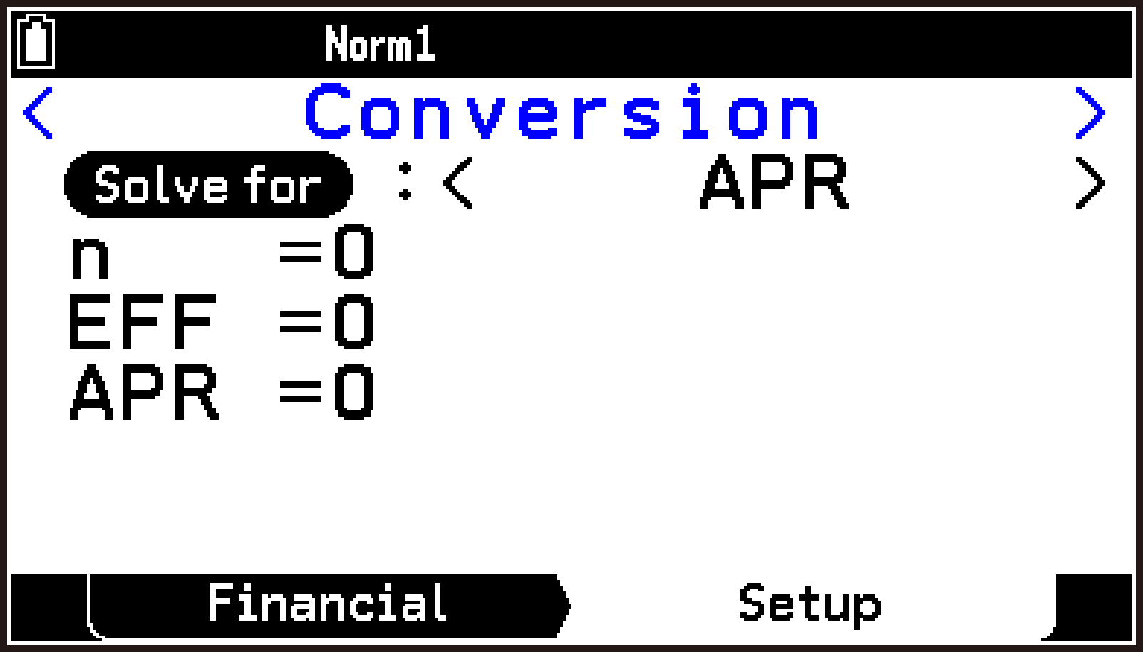
d6E5E
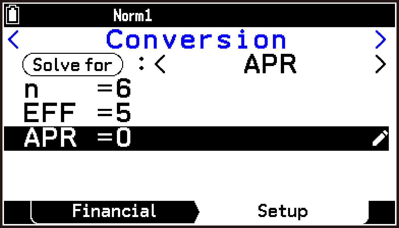
This moves the highlighting to the APR line and displays the calculation result for the annual percentage rate.
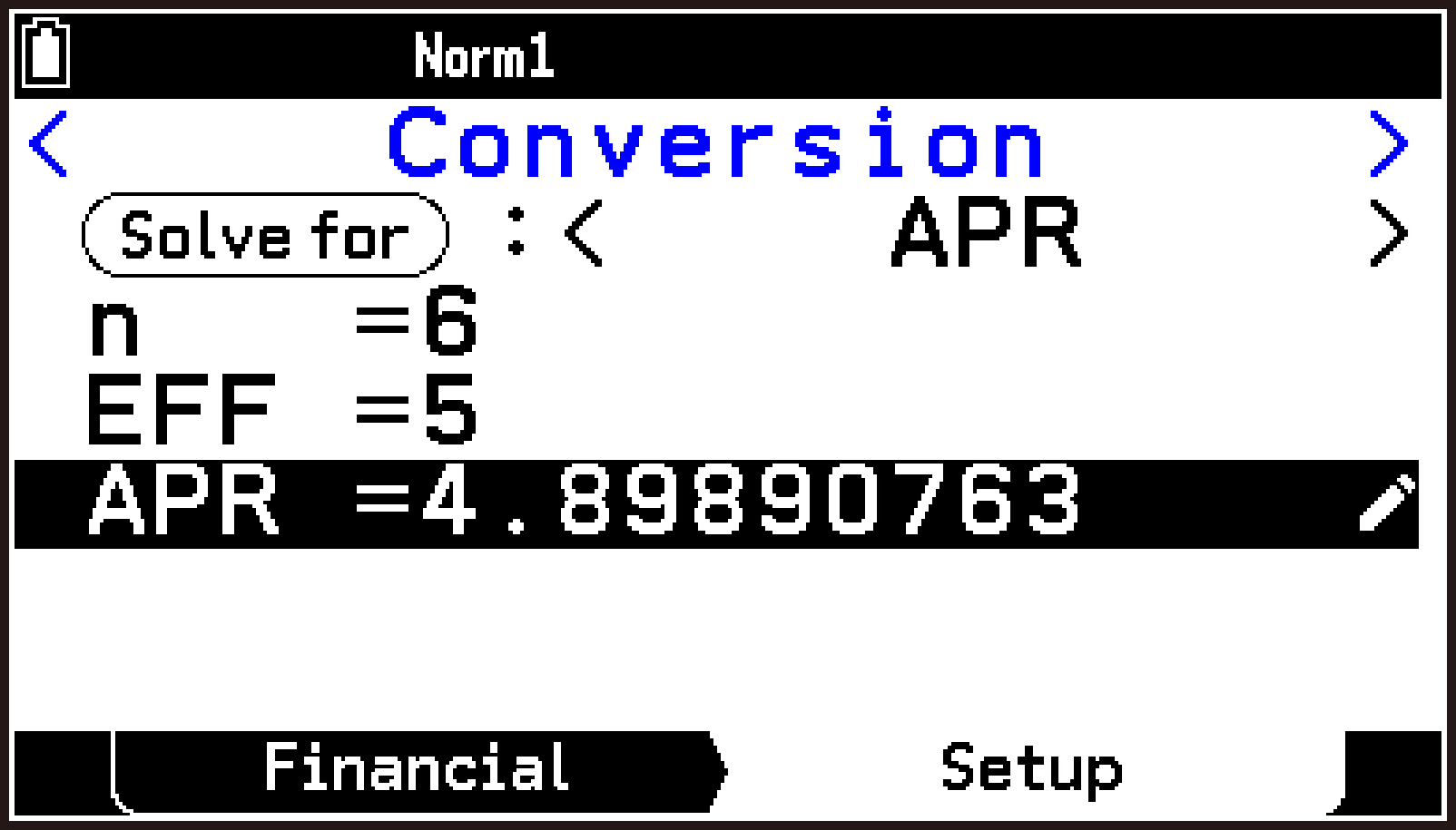
Note
You can also use the procedure below instead of step 2 above.
-
Select T > [Solve for].
-
Use d or u to select [Annual Percent Rate], and the press O.
The EFF and APR lines are used for both inputting values and displaying results.
When you select the APR item to calculate the annual percentage rate as the above example, the calculation result is displayed in the APR line based on the values entered in the n and EFF lines.
If you select the EFF item to calculate the effective interest rate, the calculation result is displayed in the EFF line based on the values entered in the n and APR lines.
Example 2 (Depreciation):
To use the sum-of-the-years’-digits method to calculate the first-year depreciation for a personal computer with a useful life (n) of 5 years and original cost (PV) of $12,000. Assume 12 months as the number of months of depreciation in the first year (Y−1). Also, display a list of the depreciation for each year.
-
On the Financial tab, highlight [Depreciation] and then press O.
-
Select the item you want to calculate.
-
Press d to highlight the
button. -
Use l or r to select the item you want to calculate.
-
Input the following information: n (useful life) = 5; PV (original cost) = 12000; FV (residual book value) = 0; j (year for calculation of depreciation cost) = 1; Y−1 (number of months in the first year of depreciation) = 12.
-
To execute the calculation, press U to highlight
, and then press O. -
To display a list of the depreciation for each year, press >.
This displays the Depreciation Setup tab.
|
To do this: |
Display this item: |
|---|---|
|
Depreciation calculation using the straight-line method (Straight-Line) |
SL |
|
Depreciation calculation using the fixed percentage method (Fixed Percent) |
FP |
|
Depreciation calculation using the sum-of-the-years’-digits method (Sum-of-the-Years’-Digits) |
SYD |
|
Depreciation calculation using the declining balance method (Declining Balance) |
DB |
|
Calculation of the depreciation rate for the fixed percentage method (Depreciation Rate (%)) |
I% |
Since we want to calculate using the sum-of-the-years’-digits method, display “SYD” here.
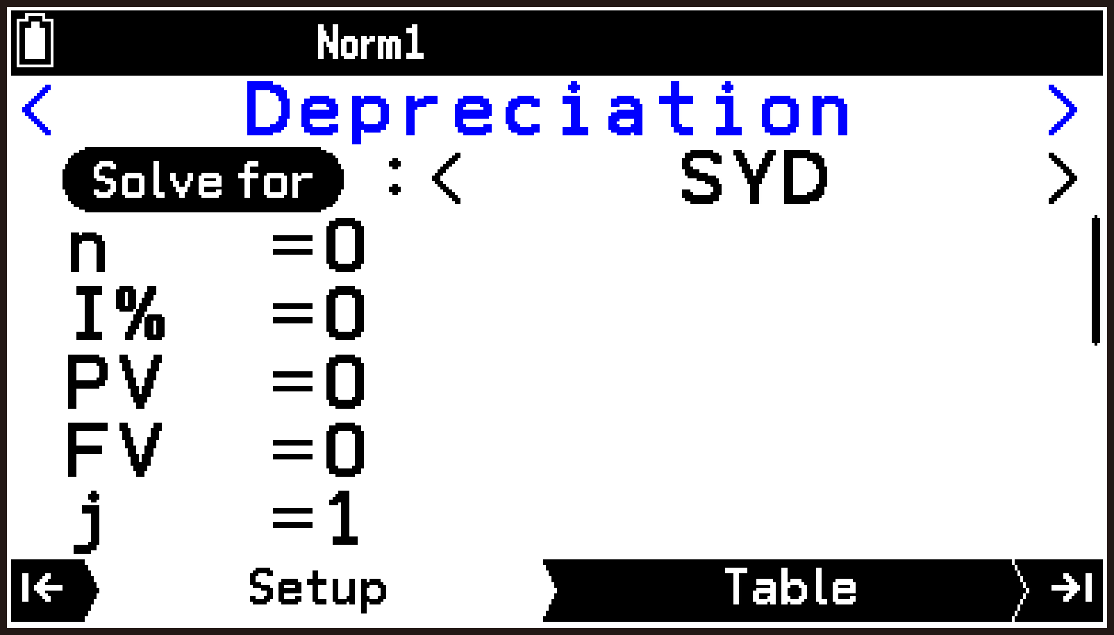
d5Ed12000E0E1E12E
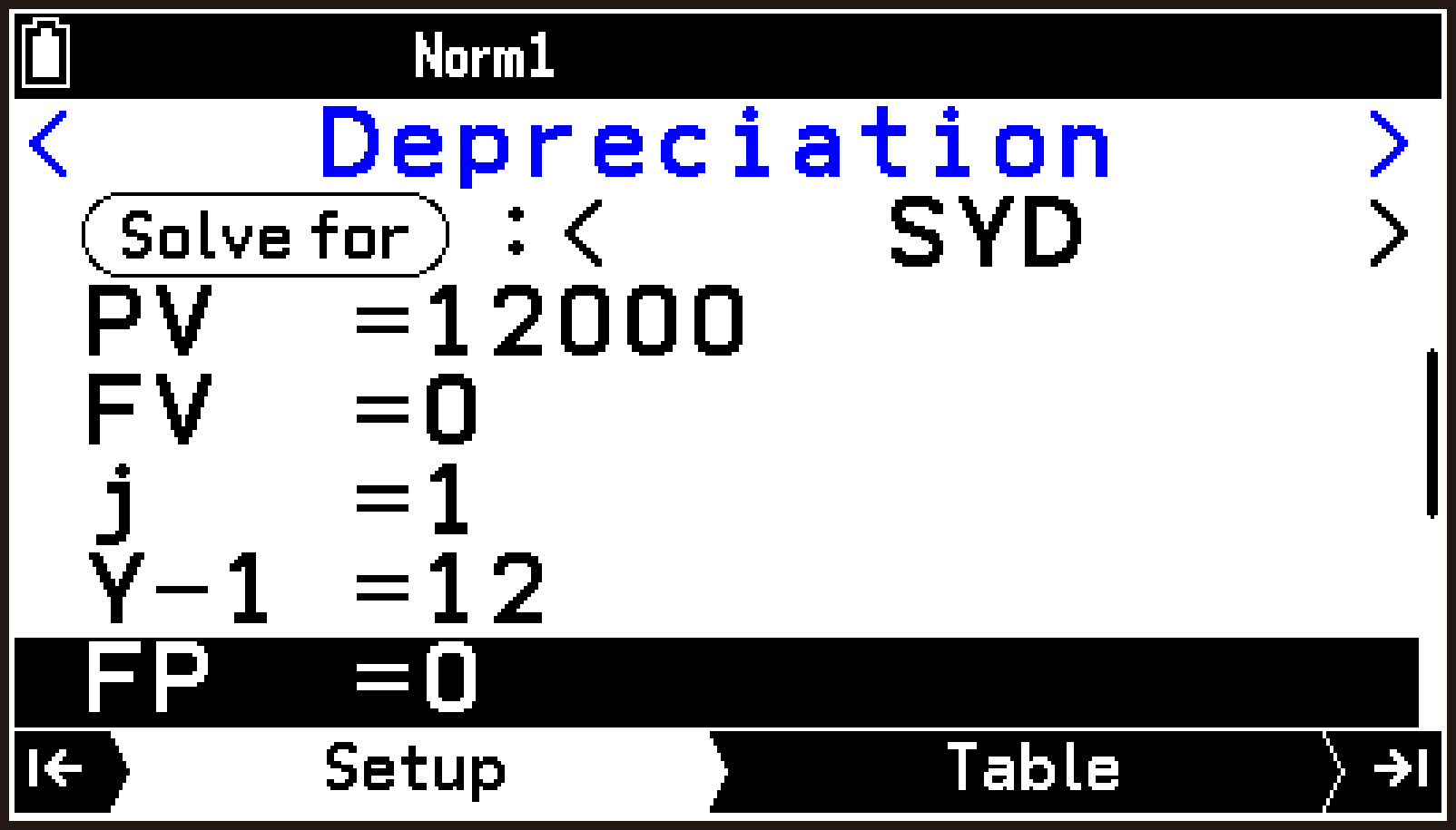
This moves the highlighting to the SYD line and displays the calculation result for the first-year depreciation.
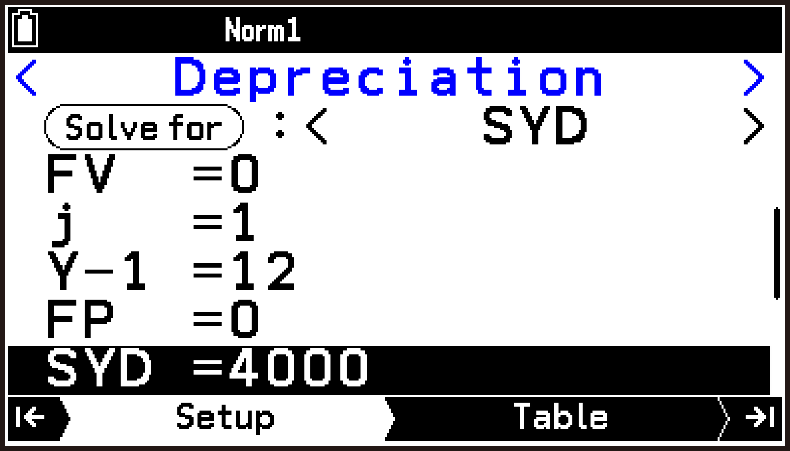
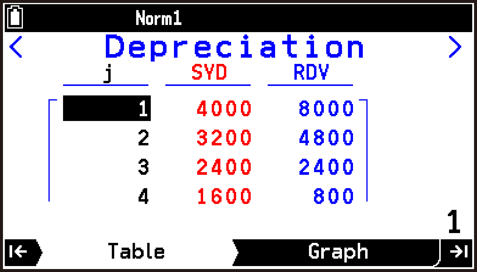
The Table tab shows the depreciation (SYD) for each year (j) and the remaining depreciated value (RDV) at the end of each year.
While viewing the Table tab, you can display the graph by pressing >.
Note
Instead of step 2 above, you can also select T > [Solve for] > [Sum-of-the-Years’-Digits].
All lines below the FP line are for displaying results only. You cannot input values in these lines.
Example 3 (Bond Calculation):
You want to purchase a semiannual bond*1 that matures on December 15, 2028 (d2) and has a settlement date of June 1, 2024 (d1). The bond is calculated based on 365 days per year.*2 The bond is redeemed at 100% of its face value (RDV) and the coupon rate (CPN) is 3%. If the yield to maturity (YLD) is 4%, determine the price of the bond (PRC), the accrued interest (INT), and the purchase price including accrued interest (CST).
S > [Interest Paid]: Semi-annually
-
On the Financial tab, highlight [Bond Calculation] and then press O.
-
Select the item you want to calculate.
-
Press d to highlight the
button. -
Use l or r to select the item you want to calculate.
-
Input the following information: d1 = 6/1/2024 (month/day/year); d2 = 12/15/2028 (month/day/year); RDV = 100; CPN = 3; YLD = 4.
-
To execute the calculation, press U to highlight
, and then press O.
This displays the Bond Calculation Setup tab.
|
To calculate this: |
Display this item: |
|---|---|
|
Bond’s Price |
PRC |
|
Yield to Maturity |
YLD |
|
Accrued Interest |
INT |
|
Dirty Price |
CST |
Since we want to determine the bond price, display “PRC” here.
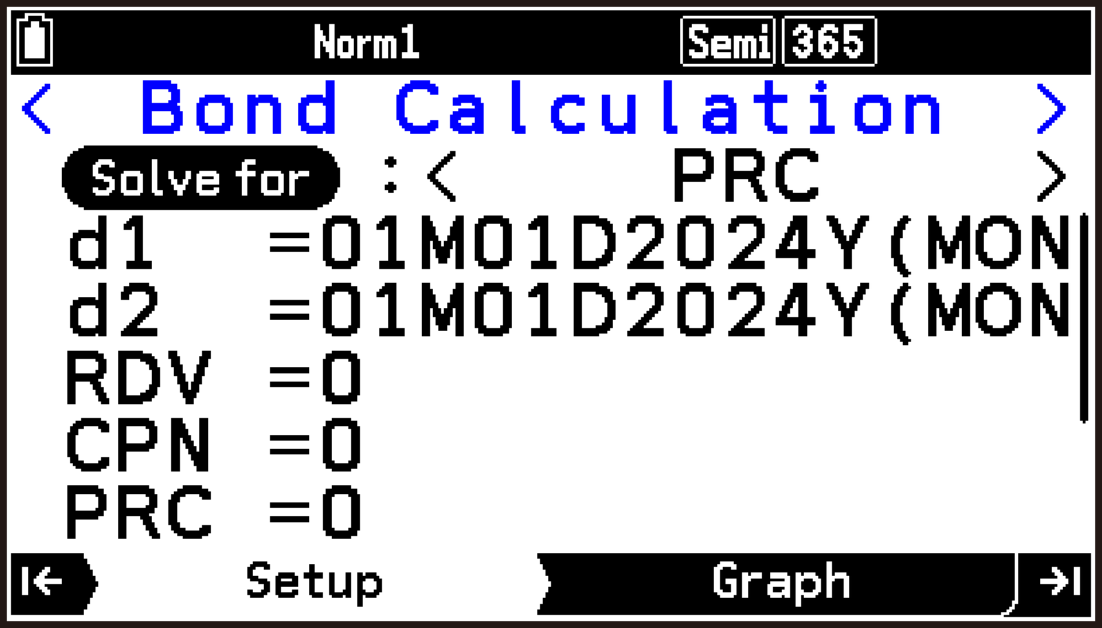
dE6E1E2024EE
E12E15E2028EE
100E3Ed4E
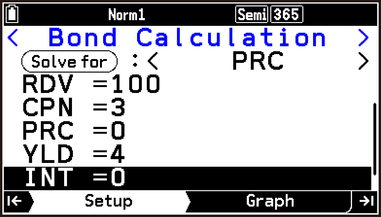
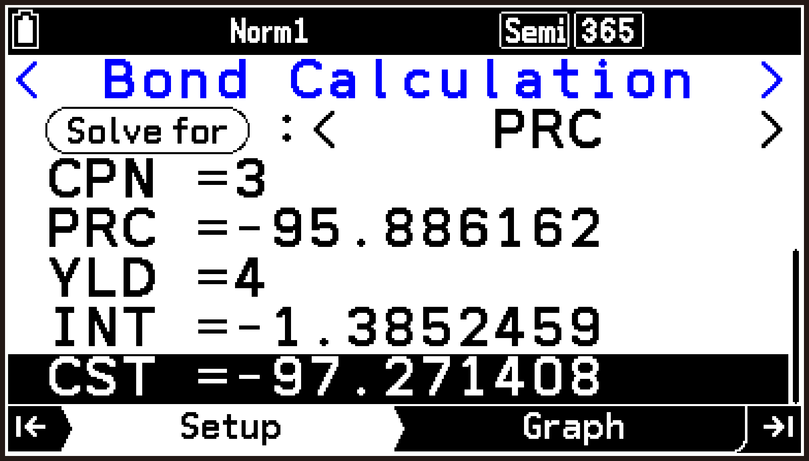
This moves the highlighting to the PRC line and displays the calculation result for the bond price.
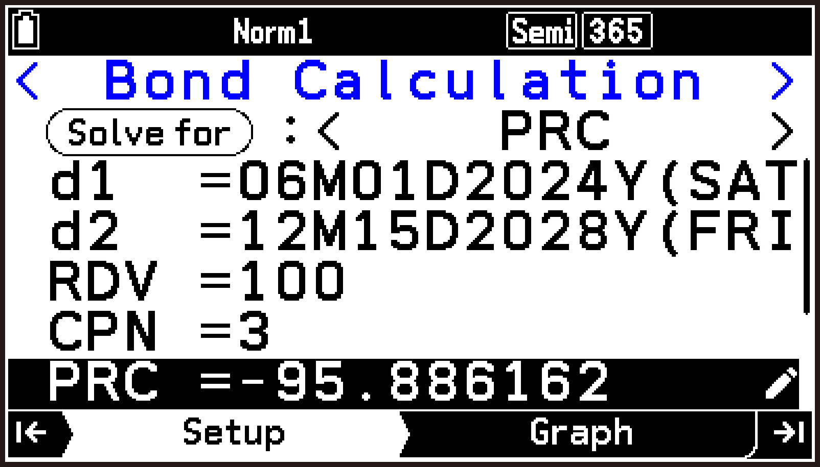
Use d to scroll the screen and display calculation results below.
PRC: bond price
INT: accrued interest
CST: price including interest
Note
Instead of step 2 above, you can also select T > [Solve for] > [Bond’s Price].
The INT and CST lines are for displaying results only. You cannot input values in these lines.
Note: Bond Calculation Memorandum Screen
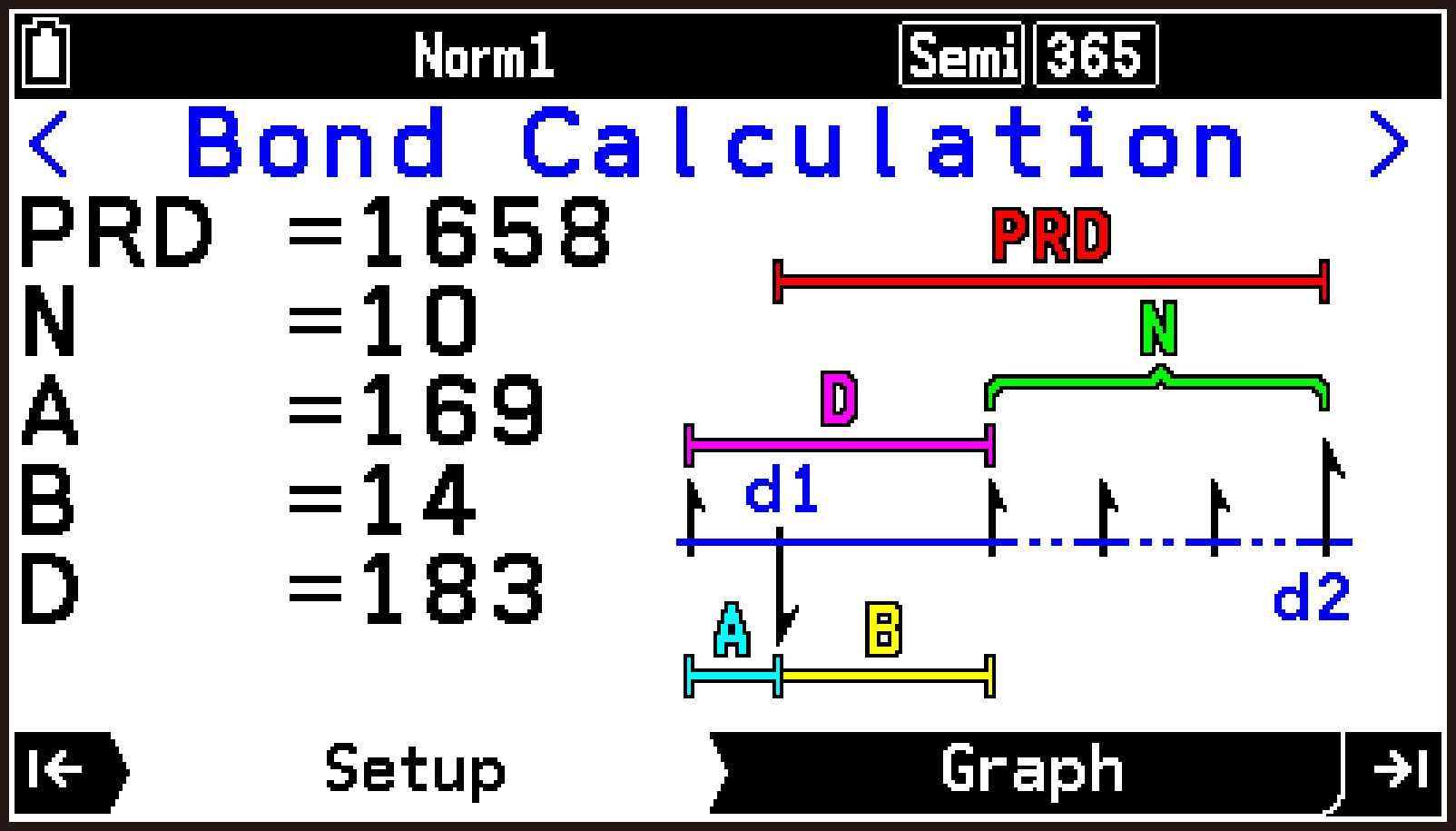
Selecting T > [Display Memorandum] on the Setup tab of Bond Calculation displays the number-of-day values used in the calculation as shown below.
PRD:
number of days from d1 to d2
N:
number of coupon payments between settlement date and maturity date
A:
accrued days
B:
number of days from settlement date until next coupon payment date (D − A)
D:
number of days in coupon period where settlement occurs
Selecting T > [Show Coupon Payment Day] while the Memorandum screen is displayed changes to a screen showing the interest payment date (only when S > [Number of Days/Year] is “365”). If there are multiple interest payment dates from the redemption year to the year of purchase, each press of O while this screen is displayed each interest payment date scrolls back sequentially until the first payment is reached.
Input/Output Terms and Calculation Formulas
Simple Interest
: interest
: number of interest periods
: principal
: annual interest rate
: principal plus interest
365-day Mode:
360-day Mode:
Compound Interest
: number of compound periods
: annual interest rate
: present value
: payment
: future value
: installment periods per year
: compounding periods per year
When calculating PV, PMT, FV, n
|
|
|
|
When S > [Payment Point] is “End” |
When S > [Payment Point] is “Beginning” |
|
0 |
1 |
|
|
When |
When and/or |
When calculating I%
(effective interest rate) is calculated using Newton’s Method.
is calculated from using the formulas below:
|
|
When |
When and/or |
Important!
When inputting both the present value (PV) and future value (FV) for a calculation, either PV or FV must be positive, while the other (PV or FV) is negative.
Annual interest rate (I%) calculations are performed using Newton’s Method, which produces approximate values whose precision can be affected by various calculation conditions. Interest calculation results produced by this application should be used keeping the above in mind, or results should be confirmed separately.
Cash Flow
This calculator uses the discounted cash flow (DCF) method to perform investment appraisal by totalling cash flow for a fixed period. This calculator can perform the following four types of investment appraisal.
: Net present value
: Internal rate of return
: Net future value
: Payback period
A cash flow diagram like the one shown below helps to visualize the movement of funds.
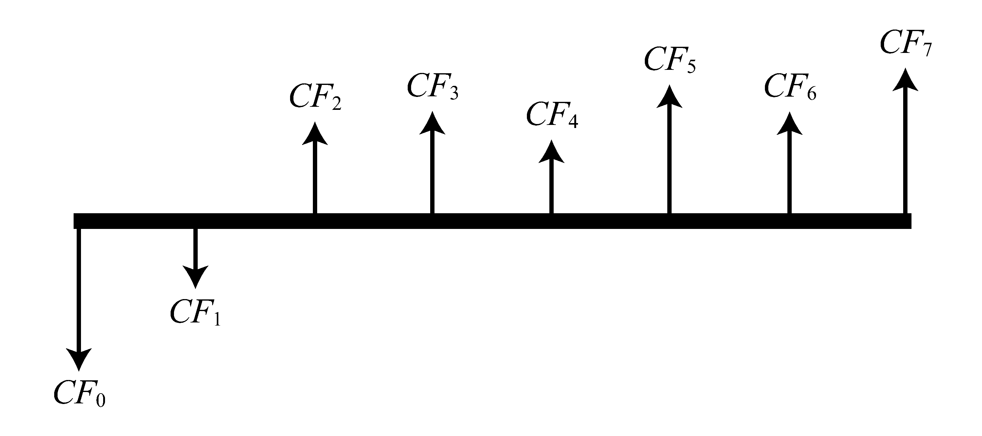
With this graph, the initial investment amount is represented by . The cash flow one year later is shown by , two years later by , and so on.
is calculated using the formula below:
In this formula, = 0, and the value of is equivalent to × 100. It should be noted, however, that minute fractional values tend to accumulate during the subsequent calculations performed automatically by the calculator, so never actually reaches exactly zero. becomes more accurate the closer that approaches to zero.
|
|
|
|
|
|
: smallest positive integer that satisfies the conditions |
Amortization
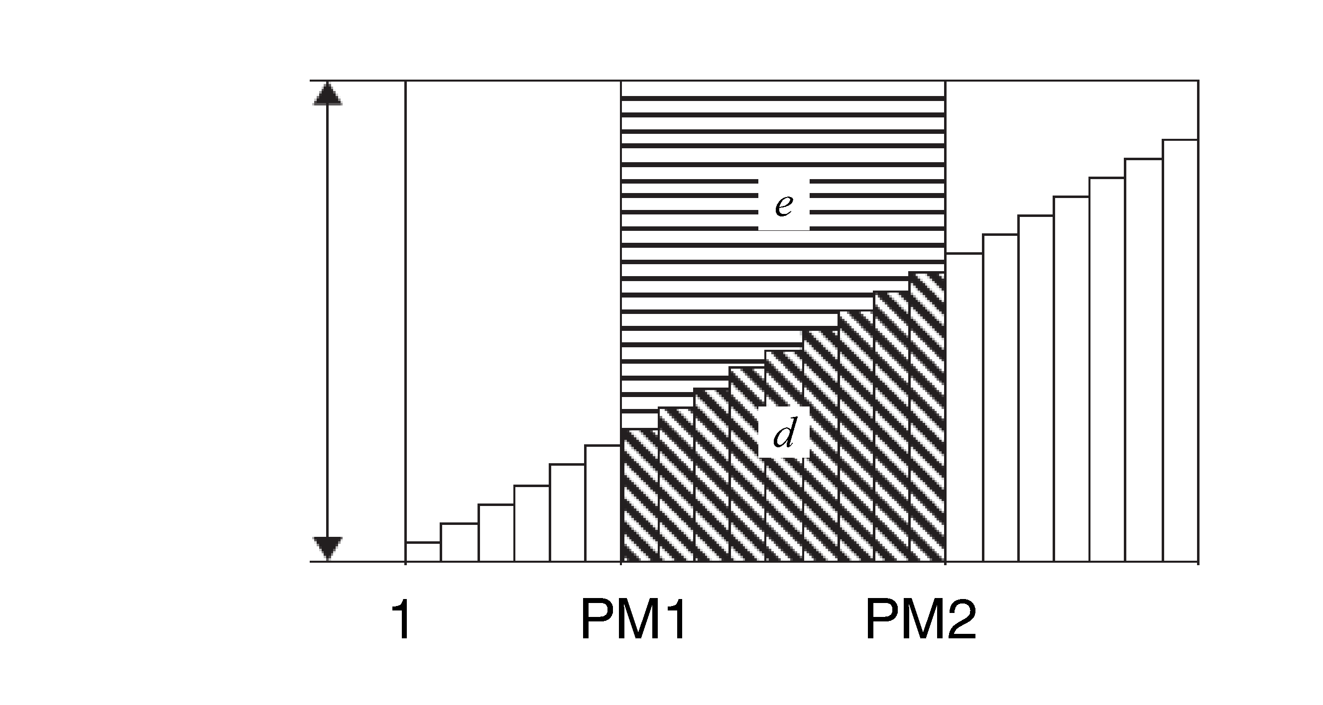
: first installment of installments 1 through
: second installment of installments 1 through
: installments
: interest rate
: principal
: payment for each installment
: balance following final installment
: installments per year
: compoundings per year
1 payment
Last
Number of payments
1 payment
Last
Number of payments
|
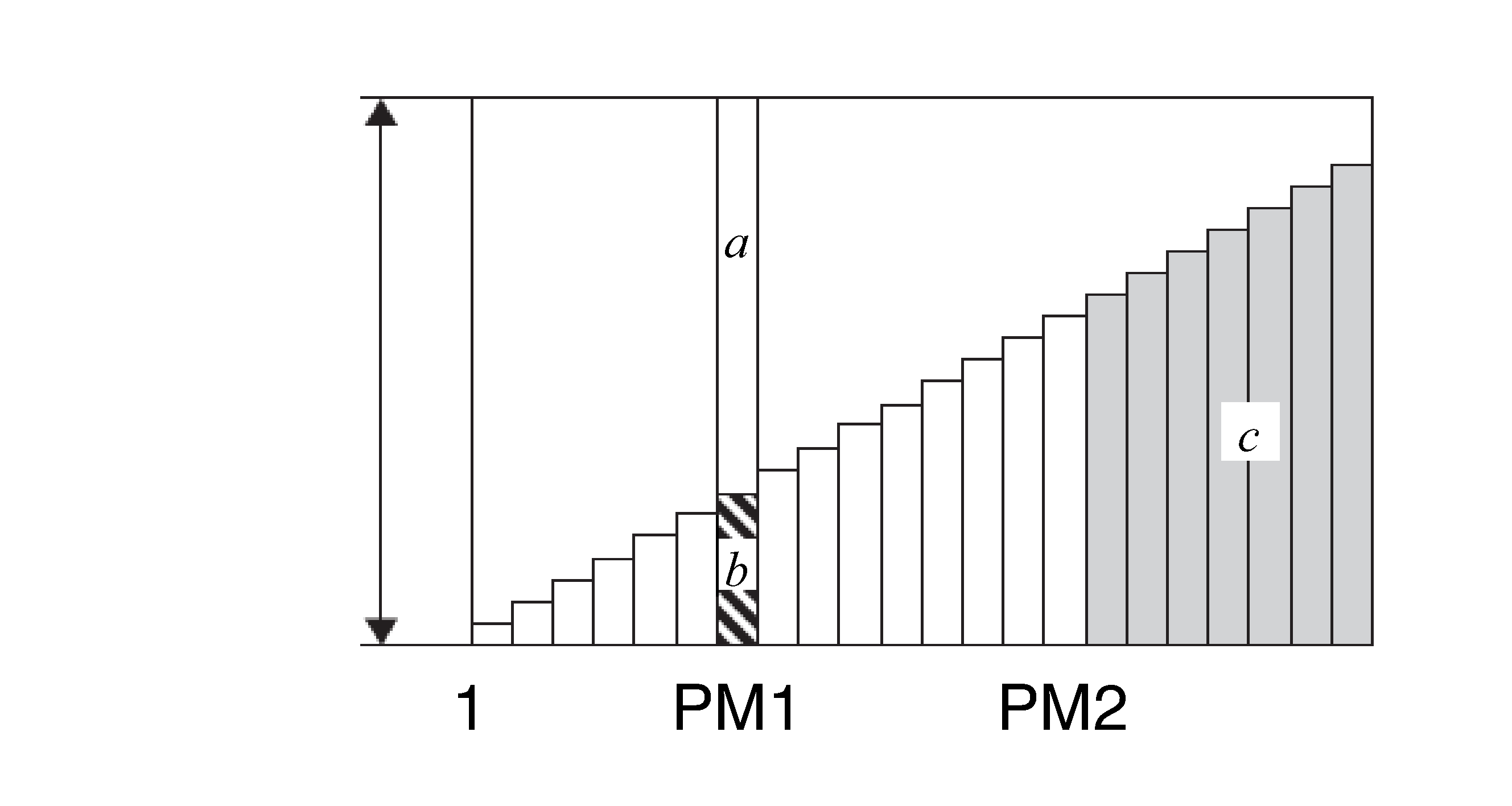
: interest portion of installment PM1 (INT) |
|
|
: principal portion of installment PM1 (PRN) |
+ = one repayment (PMT)
|
: balance of principal after installment PM2 (BAL) |
|
|
: total principal from installment PM1 to payment of installment PM2 (ΣPRN) |
|
|
: total interest from installment PM1 to payment of installment PM2 (ΣINT) |
When S > [Payment Point] is “End”, .
When S > [Payment Point] is “Beginning”, and .
Converting between the nominal interest rate and effective interest rate
The nominal interest rate (I% value input by user) is converted to an effective interest rate (I%’) for installment loans where the number of installments per year is different from the number of compound interest calculation periods.
The following calculation is performed after conversion from the nominal interest rate to the effective interest rate, and the result is used for all subsequent calculations.
Conversion
: Effective interest rate (%)
: Annual percent rate (%)
: number of compoundings
Cost/Sell/Margin
: Cost price
: Selling price
: Margin (%)
Days Calculation
|
Number of Days |
= |
d2−d1 |
(d1: date 1, d2: date 2) |
|
Days After |
= |
d1+D |
(d1: date, D: number of days) |
|
Days Before |
= |
d1−D |
(d1: date, D: number of days) |
Depreciation
Straight-Line Method (SL)
: depreciation charge for the th year
: useful life
: original cost (basis)
: residual book value
: year for calculation of depreciation cost
: number of months in the first year of depreciation
Fixed-Percent Method (FP)
: depreciation charge for the th year
: remaining depreciable value at the end of th year
: depreciation ratio
Sum-of-the-Years’-Digits Method (SYD)
: depreciation charge for the th year
: remaining depreciable value at the end of th year
|
|
||||
Declining-Balance Method (DB)
: depreciation charge for the th year
: remaining depreciable value at the end of th year
: depreciation factor
Bond Calculation
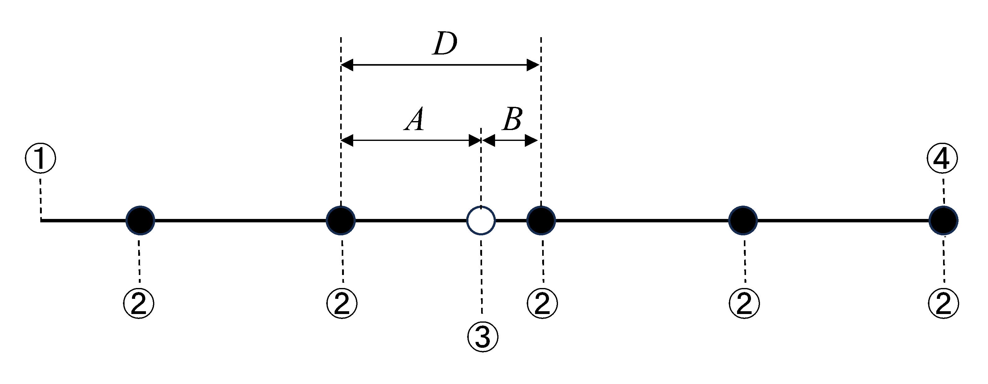
-
Issue date
-
Coupon payment dates
-
Purchase date (d1)
-
Redemption date (d2)
: price per $100 of face value
: coupon rate (%)
: annual yield (%)
: number of coupon payments per year (1=annual, 2=semi annual)
: number of coupon payments between settlement date and maturity date
: redemption price or call price per $100 of face value
: accrued interest
: price including interest
: number of days in coupon period where settlement occurs
: accrued days
: number of days from settlement date until next coupon payment date
For one or fewer coupon period to redemption
For more than one coupon period to redemption
|
|
||
Important!
The Financial app performs annual yield (YLD) calculations using Newton’s Method, which produces approximate values whose precision can be affected by various calculation conditions. Because of this, annual yield calculation results produced by this app should be used keeping the above in mind, or results should be confirmed separately.
Financial App Settings Menu Items
The Settings menu items described below are specific to the Financial app.
|
S > [Payment Point] ... |
Specifies the beginning of the period (Beginning) or the end of the period (End) as the payment date. This setting affects Compound Interest and Amortization calculations. |
|
S > [Number of Days/Year] ... |
Specifies the number of days in a year as 365 or 360. This setting affects Simple Interest, Days Calculation and Bond Calculation. |
|
S > [Interest Paid] ... |
Specifies the interval between interest payments in a Bond Calculation as either once a year or once every six months. |