E-CON5 App (Data Logger Controller)
The E-CON5 app is a dedicated controller for the CMA CLAB data logger. CLAB can use its built-in accelerometer and a variety of external sensors that can be connected to CLAB (voltage sensor, temperature sensor, motion sensor, etc.) to measure various phenomena, and then collect and store the measured data.
The E-CON5 app provides the following functions:
Configuration of measurement methods
Automatic recognition of sensors and manual configuration of sensors
Collection of data measured by sensors
Display and analysis of measured data using graphs and tables
Saving of measured data to a list variable or CSV file
Saving of measurement setups (including sensor settings, measurement method settings, and graph drawing settings) to a file, and management of saved setups
Important!
To use the E-CON5 app, the calculator must be connected to CLAB. Use the dedicated 2.5 mm plug cable to connect the calculator and CLAB. This cable is included in the optional SB-2000 (a set consisting of a USB cable and 2.5 mm plug cable).
For proper operation, you must update CLAB’s firmware to the latest version. For CLAB product information and firmware, visit the CMA website.
https://cma-science.nl/
This section assumes that you are already familiar with CLAB precautions, terminology, and operations. For details about CLAB, refer to the instruction manual included with CLAB or visit the CMA website.
Introduction
Connecting the Calculator and CLAB
-
Turn on the calculator, select h > E-CON5, and then start the E-CON5 app.
-
Use the 2.5 mm plug cable to connect the calculator’s 2.5 mm jack to CLAB’s CASIO GC jack.
-
Press the CLAB power button to turn it on.
-
Connect the temperature sensor included with CLAB to CLAB sensor terminal 1.
This displays the E-CON5 app top screen.
If “CLAB disconnected” appears on the calculator, it means CLAB is not connected to the calculator.
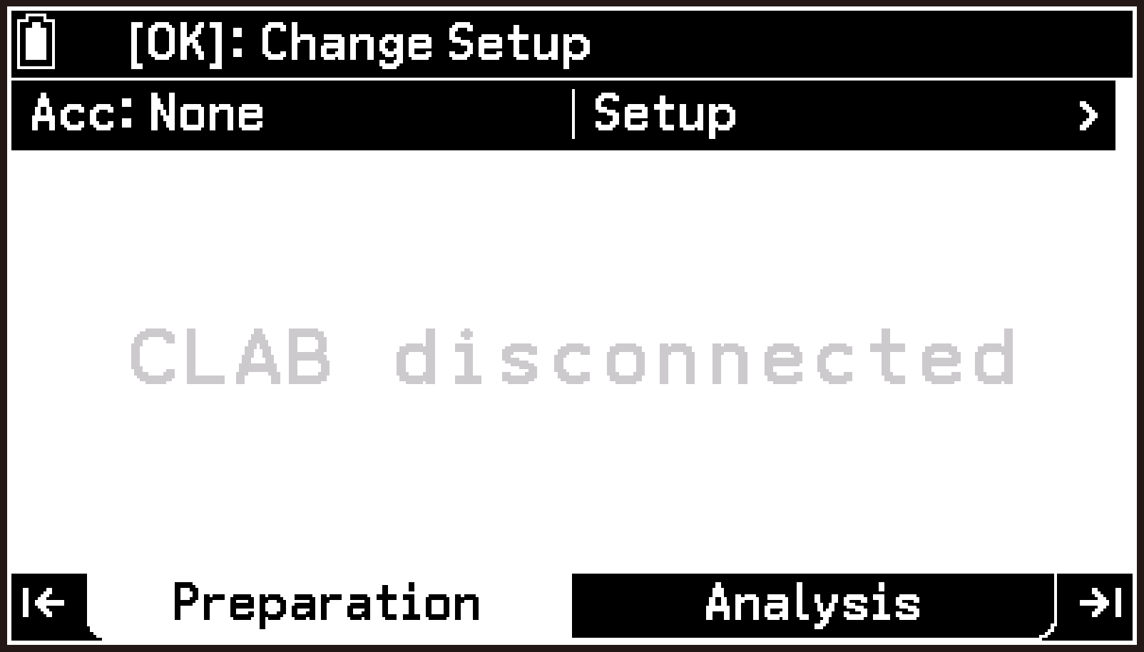
Make sure both cable plugs are firmly inserted into the calculator and CLAB jacks.
The LED on the left half of the CLAB power button flashes red, a beep sounds, and the LED lights green when the unit becomes ready for use.
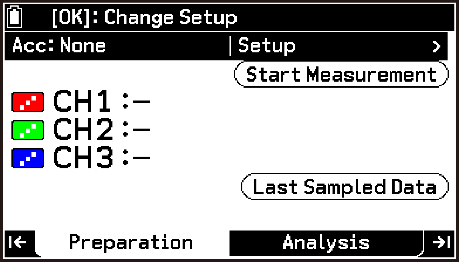
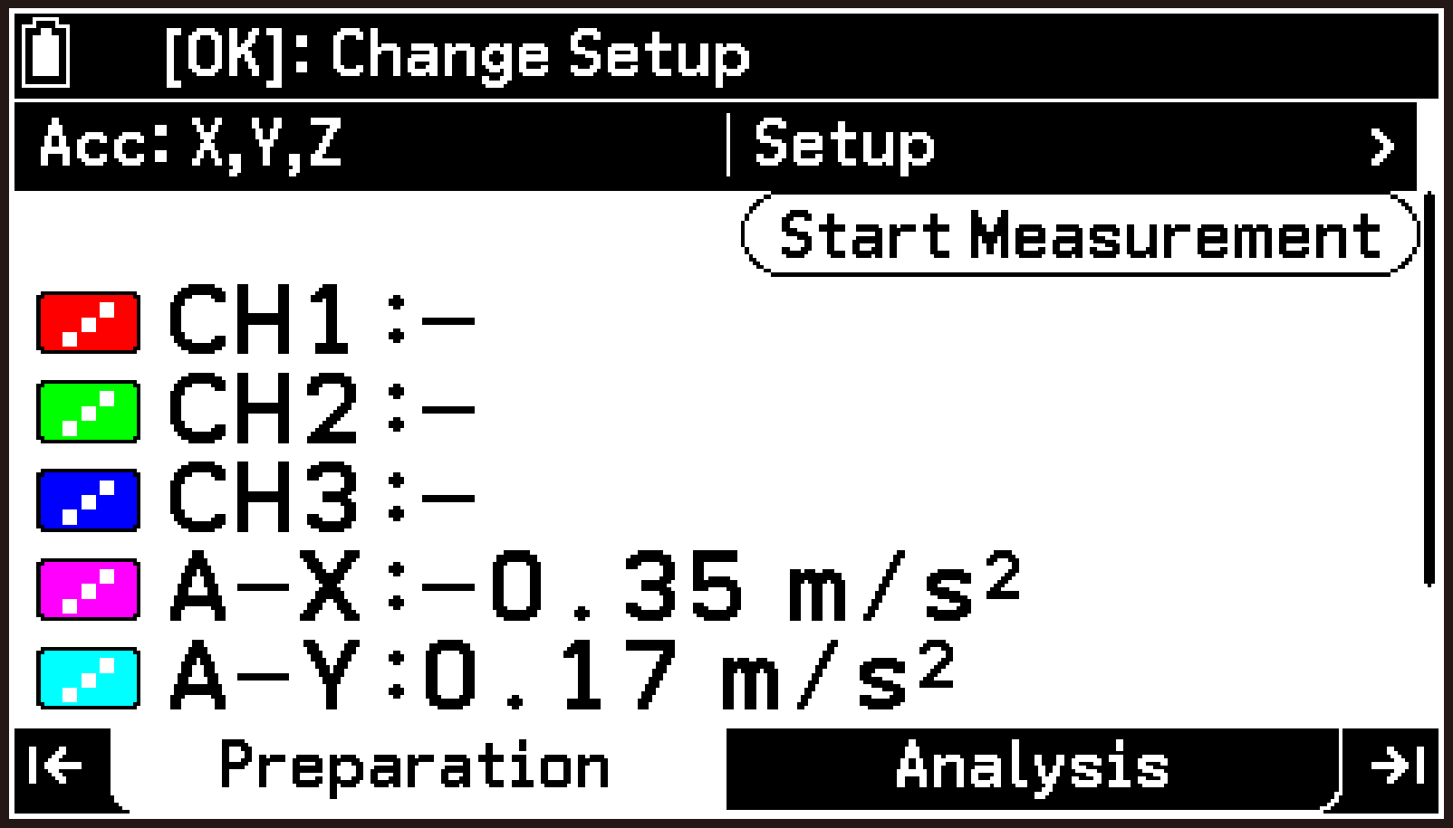
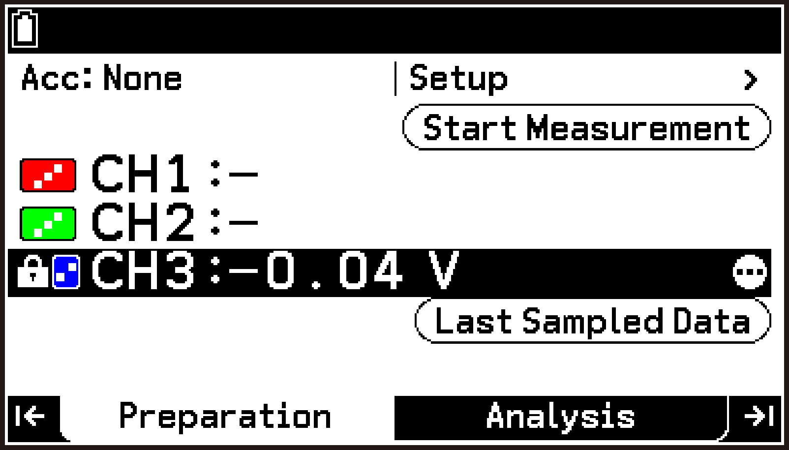
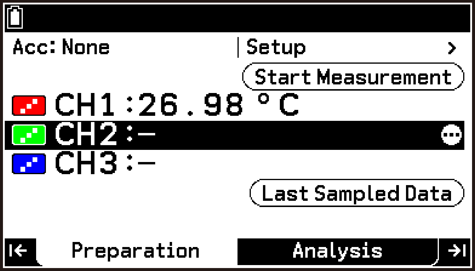
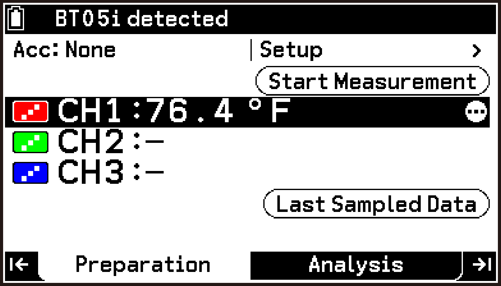
When communication between the calculator and CLAB is established, the top screen shows the input status from CLAB. The screen to the right shows that nothing is connected to CLAB sensor terminals 1, 2, or 3 (corresponding to CH1, CH2, CH3) and that there is no input from CLAB.
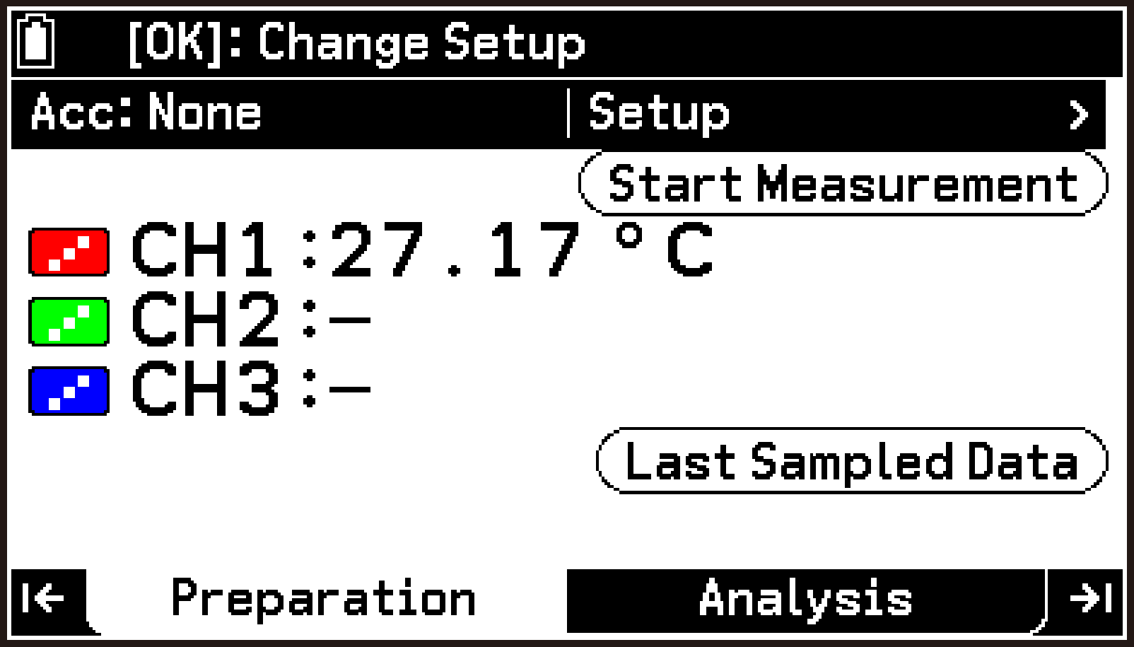
The connected sensor is recognized automatically, and the measurement value from the temperature sensor appears in the CH1 row.
Use d to highlight the CH1 row. This causes the sensor name to appear in the status bar.
Note
You can perform steps 1 through 3 above in any order. If “CLAB disconnected” appears on the calculator even after you complete all steps, there is a problem with communication between the calculator and CLAB. In this case, check again to make sure the two ends of the cable are firmly inserted into the calculator and CLAB jacks. When the connection is correct, the screen appears as shown in step 3 above.
The E-CON5 app supports sensors from CMA and Vernier. However, some sensors may not be recognized automatically when connected to CLAB. To use a sensor that is not recognized automatically, select it from the library or create a custom sensor. For details, see the information at the following locations.
To measure using CLAB’s built-in accelerometer, you must use the E-CON5 app to enable the accelerometer. For details, see Using the Acceleration Sensor.
E-CON5 App Tabs
The E-CON5 app has two tabs: the Preparation tab and the Analysis tab.

Preparation tab (Top screen)
Analysis tab (Graph screen)
Preparation Tab
Use this tab for operations related to preparing CLAB measurements, such as configuring measurement methods, configuring sensors manually, and managing setups.
The screen that first appears when you start the E-CON5 app on this tab is called the top screen. When CLAB is connected to the calculator, the measurement values from the sensors are displayed on the top screen in real time.
Analysis Tab
Use this tab to display measured data (in graphs or tables), and to analyze, and save measured data. Each time a measurement executed with CLAB and the calculator is complete, the graph screen appears on this tab.
Note
Normally, you can use < and > to move between the two tabs (except when a menu, dialog, or specific screen is displayed). You can also highlight  on the Preparation tab and press O to display the Analysis tab (graph screen).
E-CON5 App Basic Operations
Changing the Measurement Method Settings
This section explains how to display the current measurement method settings and change some of them. Here, we will change the Frequency (sampling frequency) setting from the initial value of 1/s (once per second) to 10/s (10 times per second).
Perform the following procedure after you perform steps 1 through 4 of the procedure under Connecting the Calculator and CLAB.
-
Highlight the first row of the top screen (the row that shows Acc) and press O.
-
On the Setup menu, select [Measurement Method].
-
Highlight [Frequency].
-
Enter 10, and then press O.
-
To close the Measurement Method screen and complete the setting operation, press b.
This displays the Setup menu.
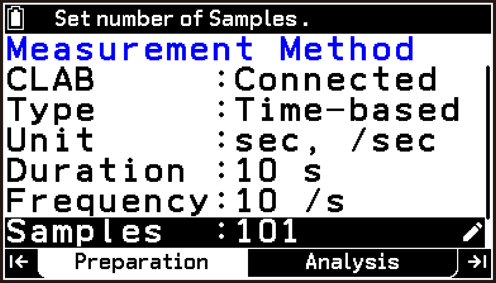
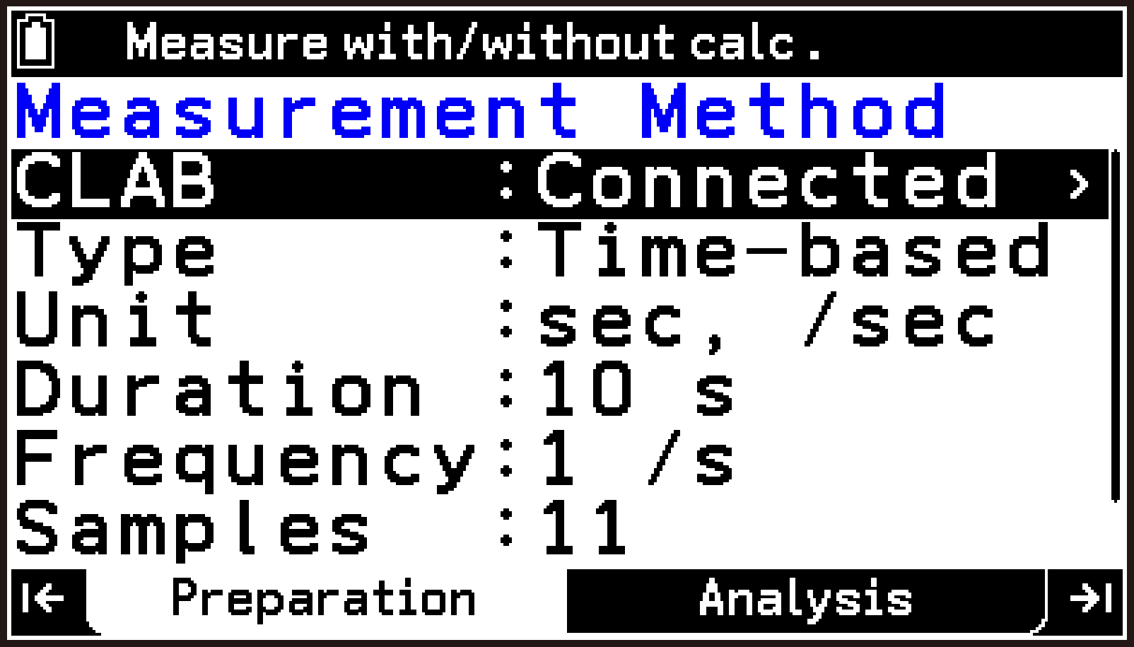
This displays the Measurement Method screen for changing to another measurement method.

The initial default items that appear in the E-CON5 app are shown in the following table.
|
Item |
Initial Default Setting |
Description |
|---|---|---|
|
CLAB |
Connected |
Specifies the CLAB operation mode. The initial default Connected mode is the operation mode in which CLAB is connected to the calculator to perform measurements. Another option is Standalone mode, which performs measurements using CLAB by itself. |
|
Type |
Time-based |
Specifies the measurement type. With the initial default Time-based type, measurement continues for the length of time specified under Duration below. |
|
Unit |
sec, /sec |
Specifies the unit for Duration and Frequency below. |
|
Duration |
10 s |
Specifies the measurement time. |
|
Frequency |
1 /s |
Specifies the sampling frequency (the number of measurements per unit of time). |
|
Samples |
11 |
Specifies the number of samples (the total number of measurements for the entire measurement time). |
|
Trigger |
None |
Specifies the measurement start condition. With the initial default None setting, measurement starts as soon as you select Start Measurement (button or menu) with the E-CON5 app. |
The items that appear on the Measurement Method screen vary depending on the CLAB operation mode and measurement type settings. For details, see Specifying the Measurement Method (Preparation Tab).
This changes the Frequency value. At the same time, the Samples value is adjusted automatically.
This returns to the top screen.
Performing a Measurement and Displaying the Results in a Graph or Table
This section shows an example of how to perform the following operations:
Perform a measurement
Display a graph of the measurement results
Change graph display settings
Display a table
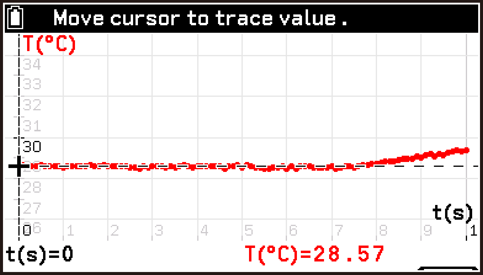
Use Trace to display coordinate values on the graph
Perform the following procedure after you perform steps 1 through 5 of the procedure under Changing the Measurement Method Settings.
Important!
When you start a measurement in step 1 of the following procedure, any previous measurement data is discarded and overwritten with the new measurement data.
-
On the top screen, highlight
 and press O.
 -
Select T > [Graph View].
-
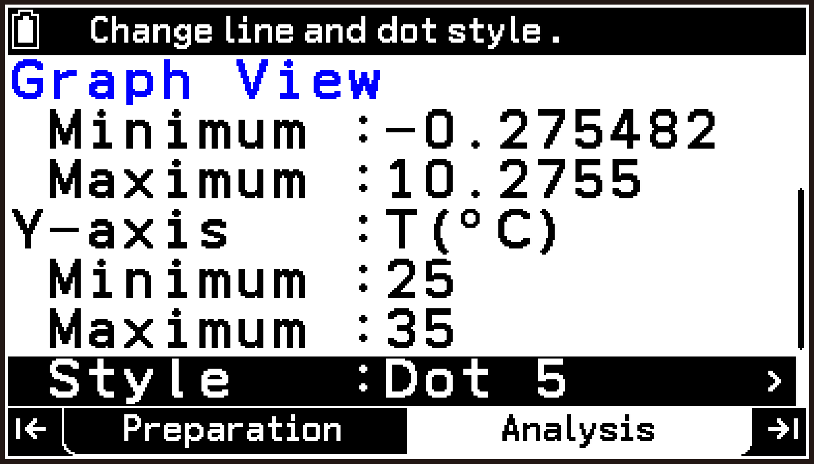
Change the Minimum of Y-axis to 25 and the Maximum to 35.
-
To return to the graph screen, press b.
-
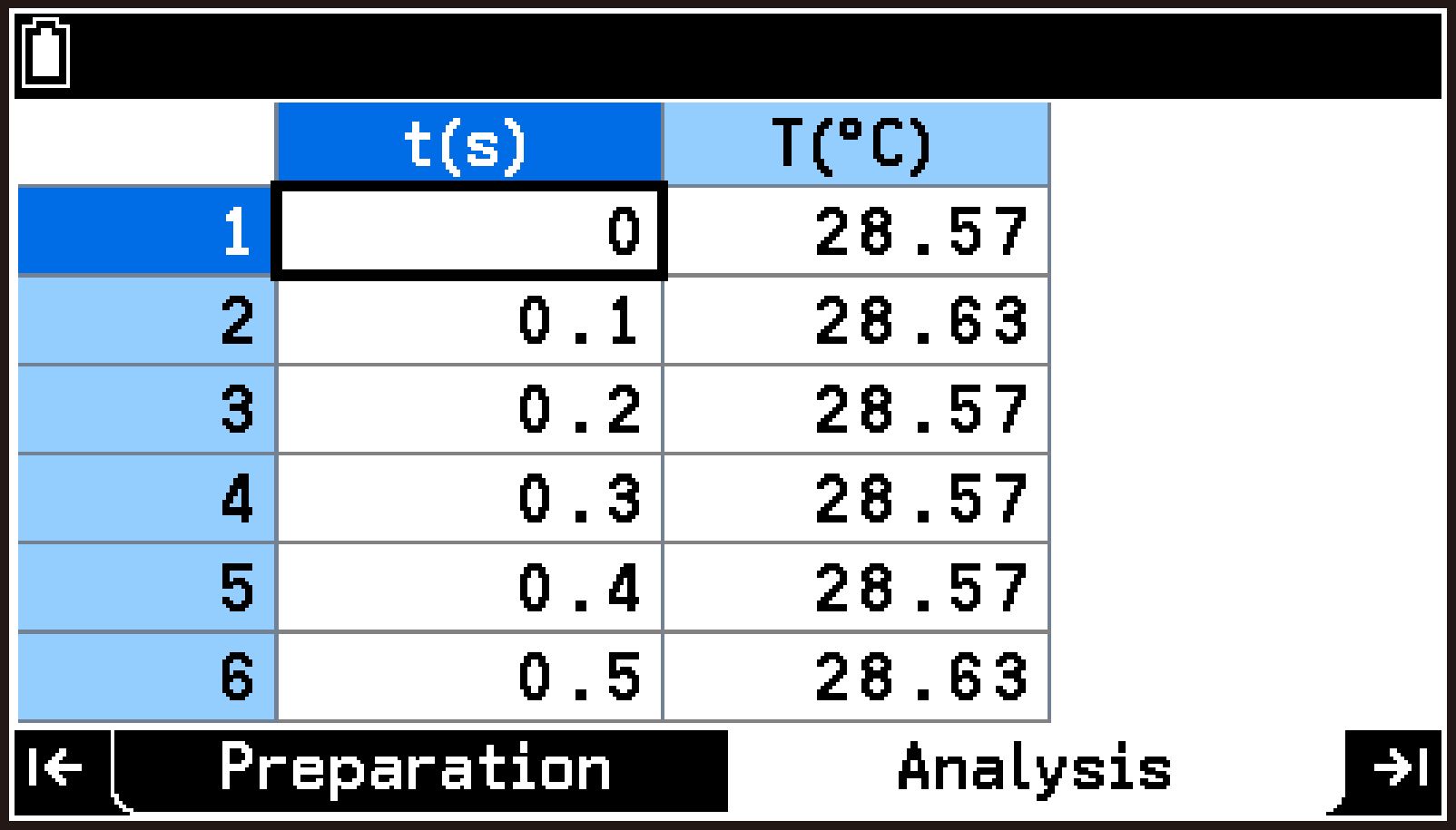
Select T > [Display Table].
-
To return to the graph screen, press b.
-
Select T > [Analyze Graph] > [Trace] to enable Trace.
-
To exit Trace, press b.
-
To return to the top screen, press < or >.
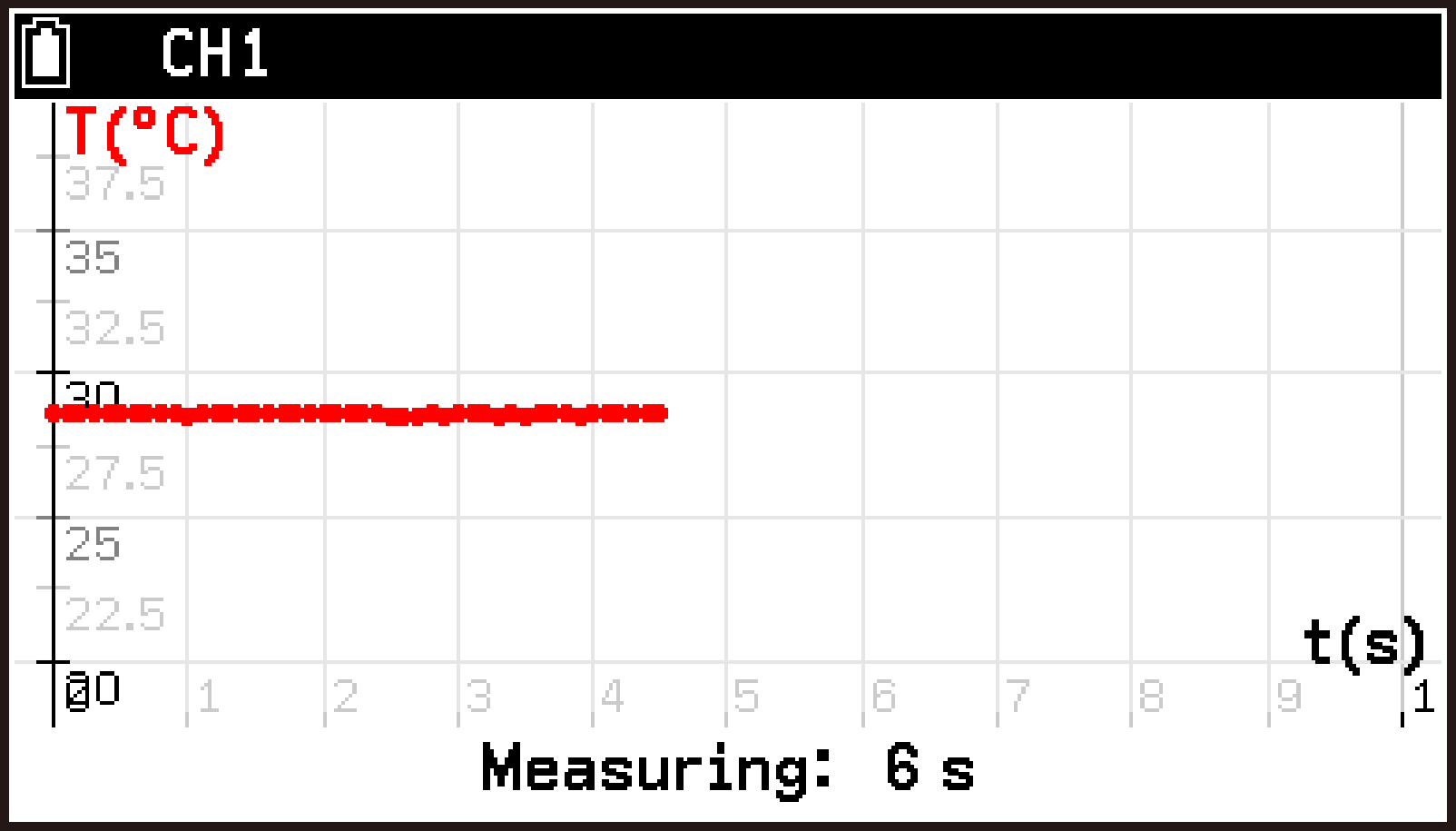
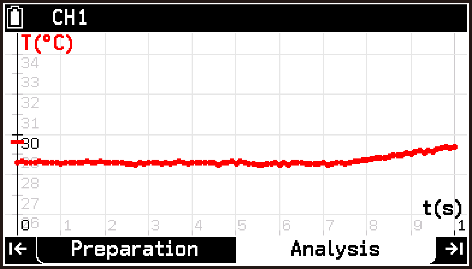
This starts measurement. While measurement is in progress, measured values appear in real time on the graph.
To interrupt measurement, press a a. See the “Note” below for more information.
Tabs do not appear until measurement ends automatically (or ends after being interrupted).
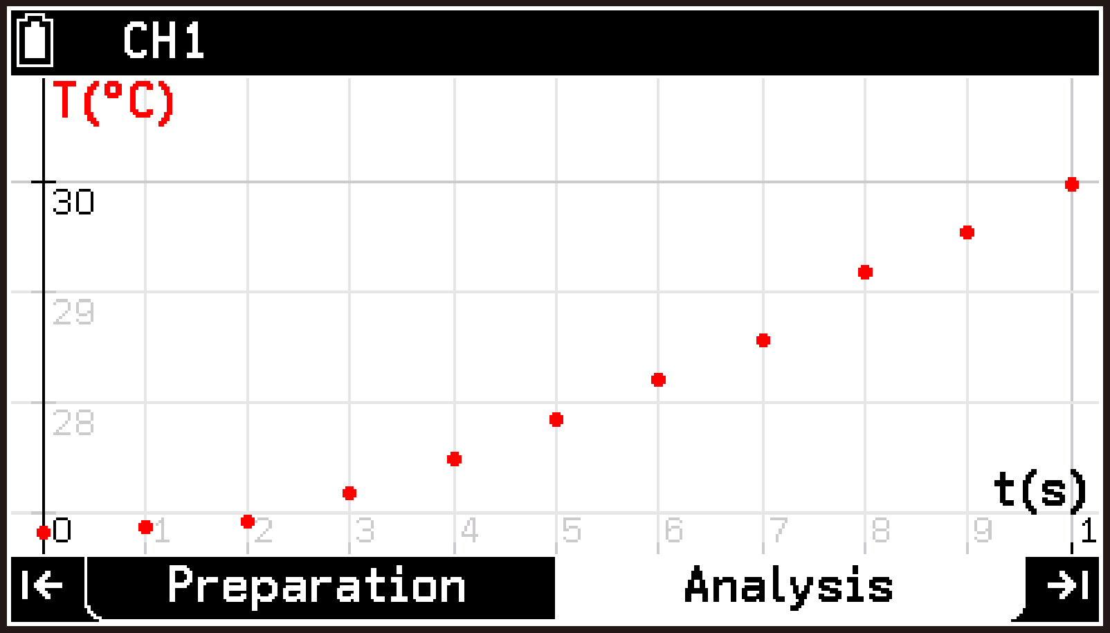
Measurement ends automatically when the specified time elapses. At this time, the Analysis tab appears with the graph screen displayed.
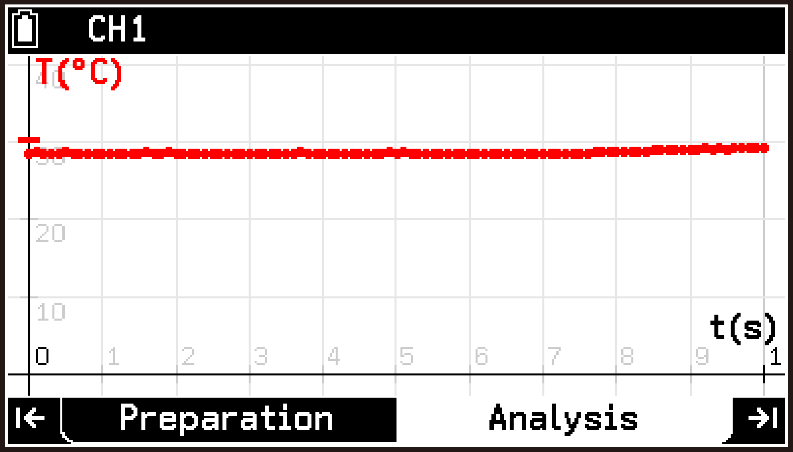
This displays the Graph View screen. You can use this screen to view and change graph display settings.
By way of example, we will change the maximum and minimum values of the graph Y-axis in step 3.
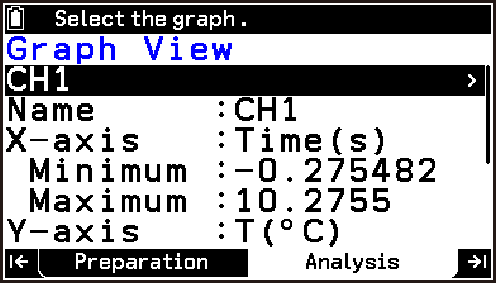
Highlight the Minimum row of Y-axis, and then enter 25. Next, highlight Maximum, and then enter 35.
The changed settings are applied to the graph screen.
For details about the items and settings on the Graph View screen, see Graph Property Settings (Analysis Tab).
This switches to the table screen.
For details about the contents of the table screen, see Table Screen Display and Menu (Analysis Tab).
A pointer (+) appears at the position of the first sample (data point) on the graph, and the coordinate values appear at the bottom of the screen.
Use l and r to move the pointer to the previous or next data point.
For details about the functions on the T > [Analyze Graph] menu, see Graph Analysis (Analysis Tab).
Note
Pressing a while measurement is in progress stops measurement and displays the following dialog.
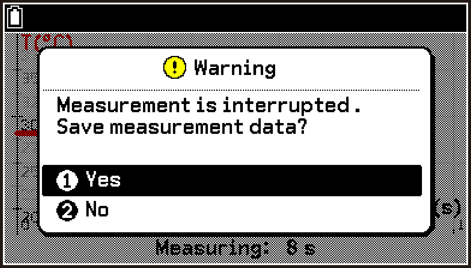
To save the measurement data collected up to the interruption, select [Yes]. If you do not want to save it, select [No]. If you select [Yes], the app displays the graph screen. Selecting [No] causes the app to return to the top screen.
On the top screen, press < or >, or highlight , and then press O. This displays the last graph screen you viewed.
To start a new measurement while the graph or table screen is displayed
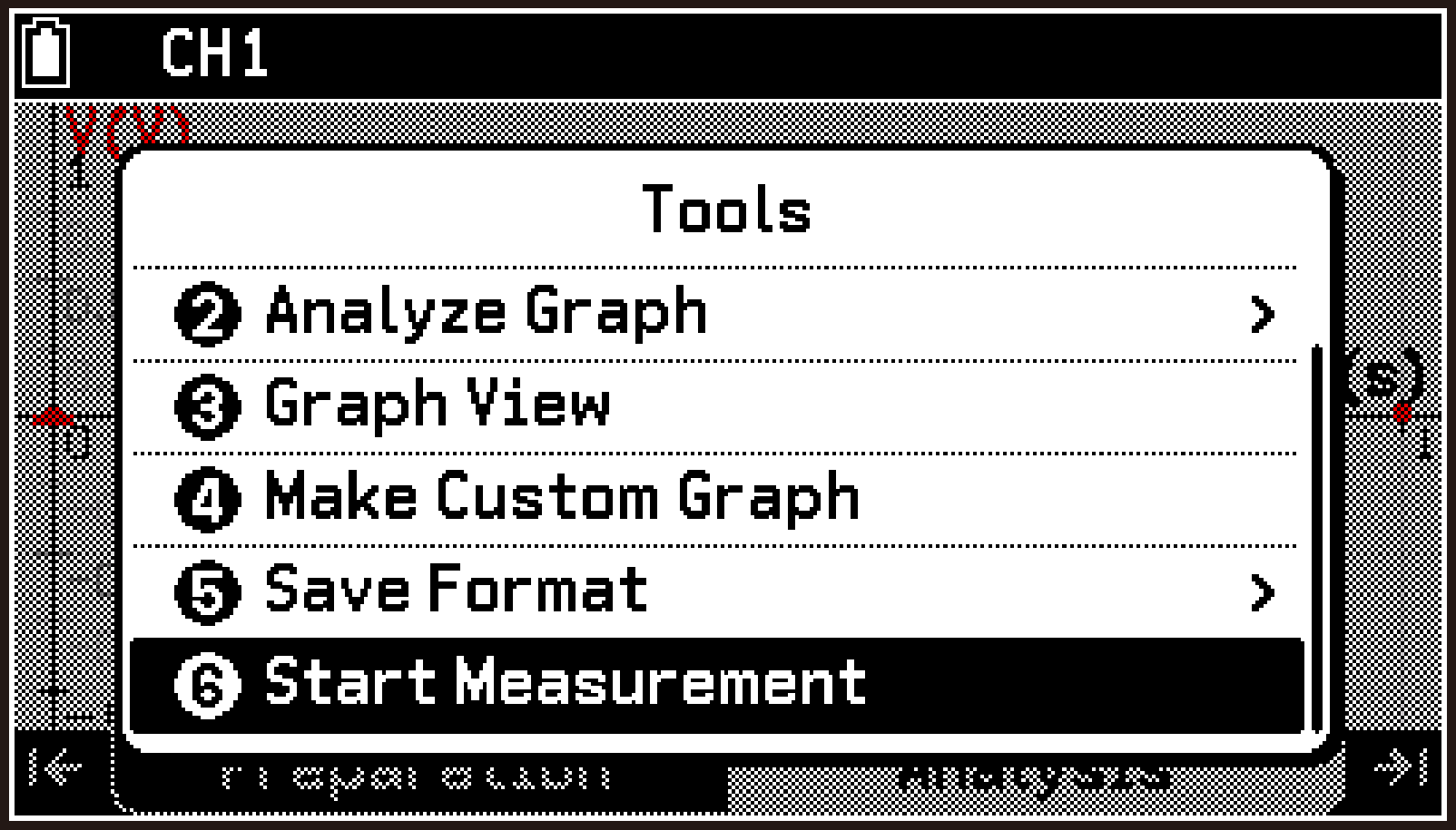
You can start a new measurement while the graph screen or table screen is displayed, without returning to the top screen. To start measurement, select T > [Start Measurement]. This operation is the same as highlighting on the top screen and pressing O.
Important!
When you select T > [Start Measurement] on the graph screen or table screen, previous measurement data is discarded and overwritten with the new measurement data.
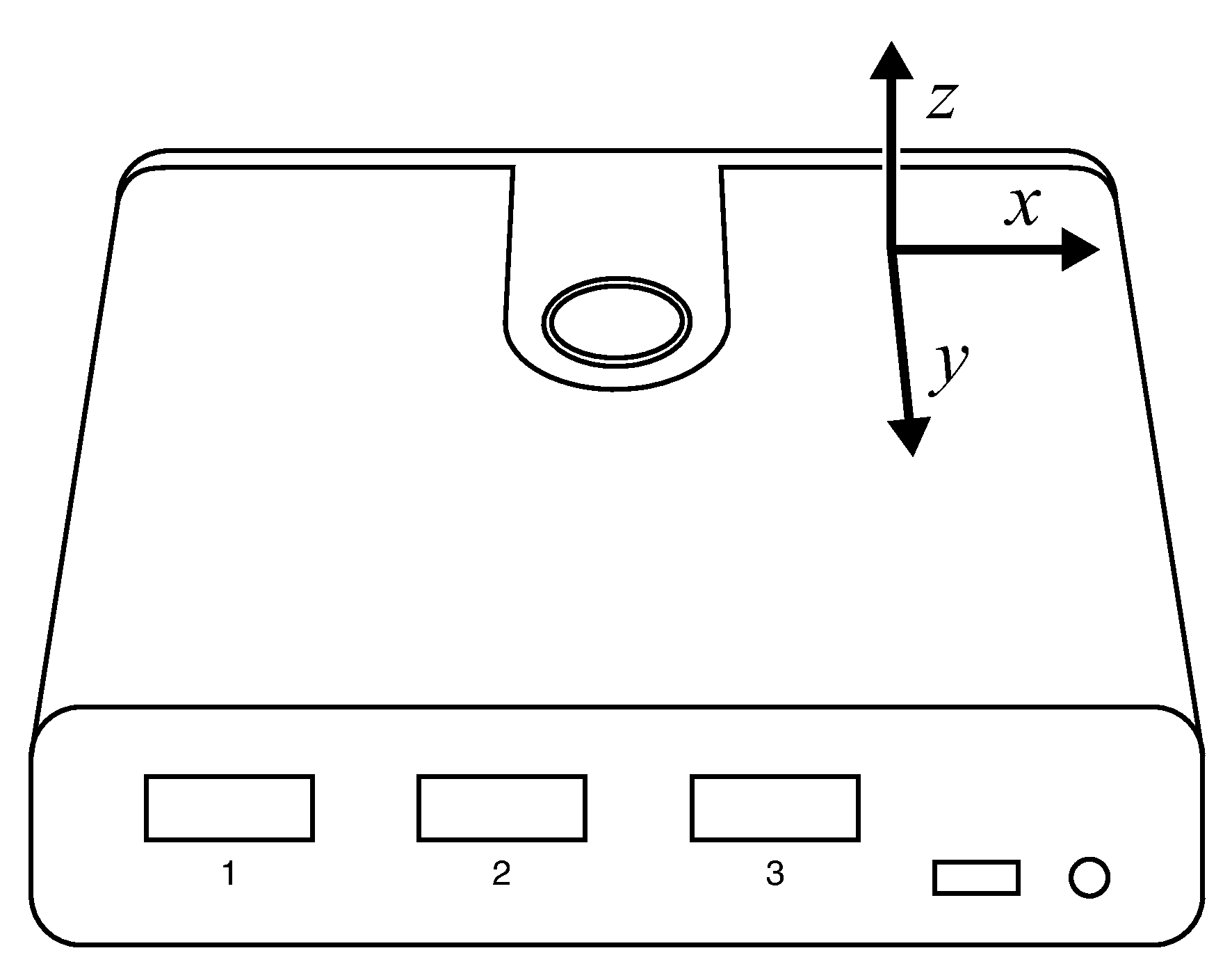
Using the Acceleration Sensor
CLAB has a built-in three-axis accelerometer. It can measure acceleration in the -axis, -axis, and -axis directions within a range of ±20 m/s2 (initial default) or ±40 m/s2.
When you hold CLAB with the surface containing the power button facing upward, the acceleration in each axis direction is approximately as follows:
-axis direction ≒ 0 m/s2
-axis direction ≒ 0 m/s2
-axis direction ≒ -9.8 m/s2
To enable the accelerometer and perform measurement
-
Connect the calculator and CLAB, and then start the E-CON5 app.
-
Highlight the first row of the top screen and press O.
-
On the Setup menu that appears, select [Accelerometer].
-
Enable all three axes of the accelerometer (
 ) and press b.
 -
Perform the procedure under Changing the Measurement Method Settings to change the settings as shown below.
-
After configuring the settings, press b to return to the top screen.
-
Highlight
and press O. -
To return to the top screen, press < or >.
This displays the E-CON5 app top screen.
Perform the following steps of this procedure with no sensors connected to CLAB sensor terminals.

This displays the Acc menu.
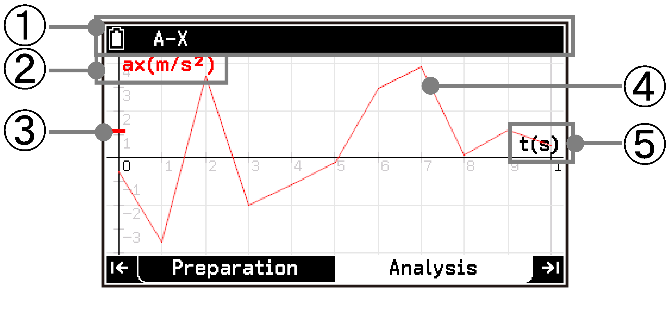
[A-X] … Enables/disables the accelerometer -axis.
[A-Y] … Enables/disables the accelerometer -axis.
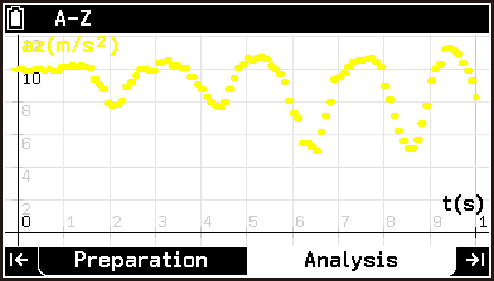
[A-Z] … Enables/disables the accelerometer -axis.
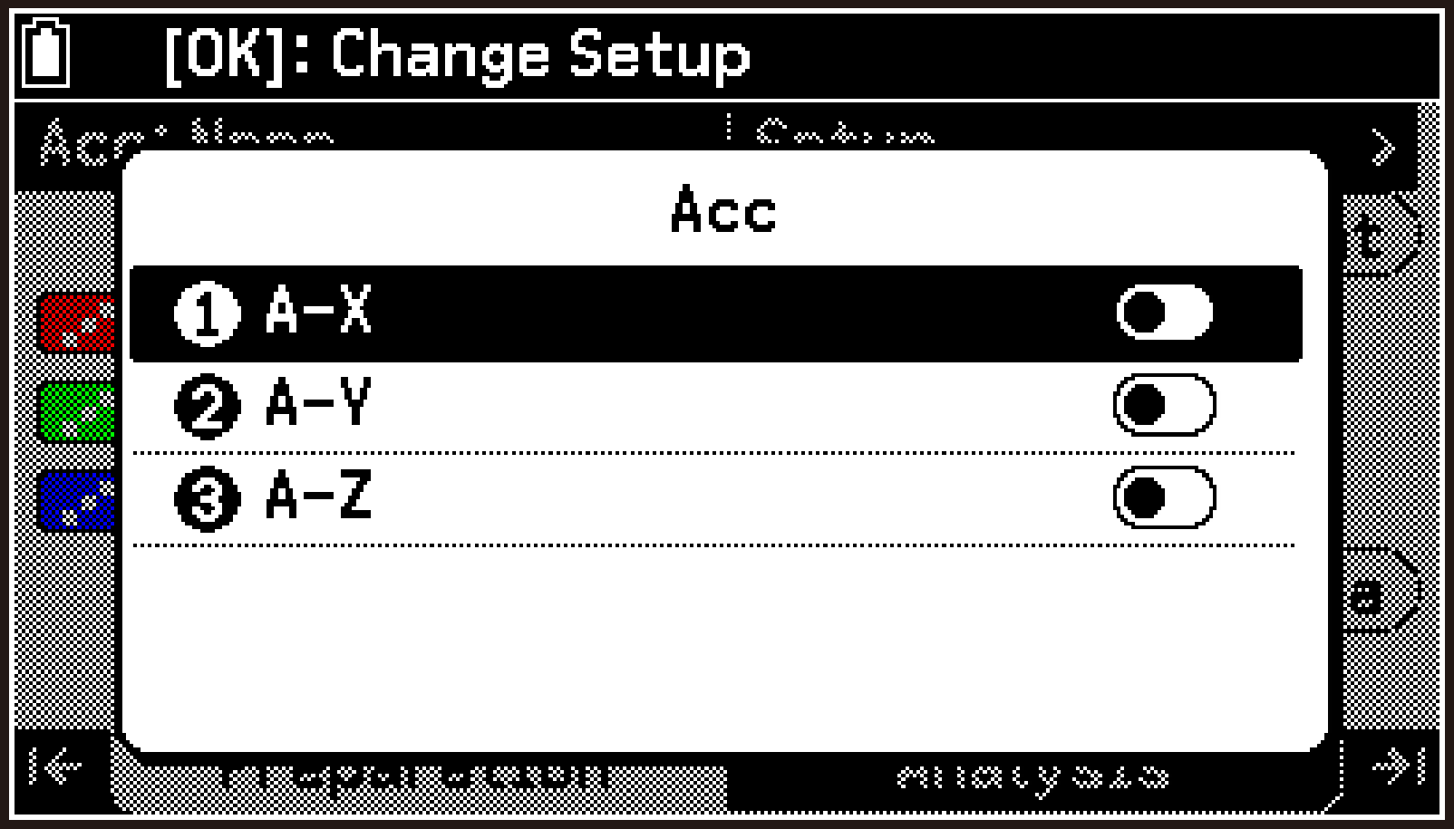
The A-X, A-Y, and A-Z rows are added to the top screen, and measured values appear in each row. (To view the A-Z row, scroll the screen.)
Now let’s actually perform a measurement using the accelerometer. Specify the measurement method in step 5 and start measurement in step 7.
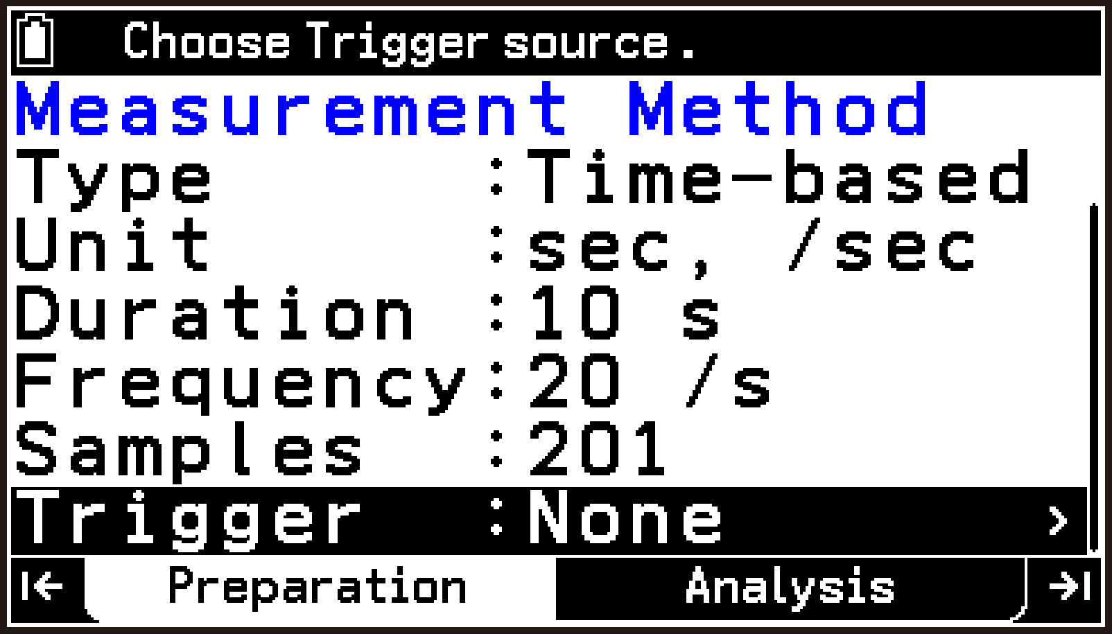
CLAB: Connected
Type: Time-based
Unit: sec, /sec
Duration: 10 s
Frequency: 20 /s
Samples: 201
Trigger: None
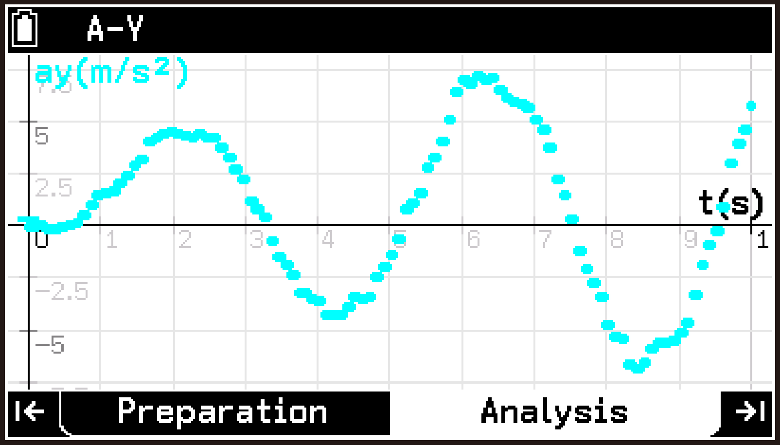
While measurement is in progress, measured values appear in real time on the graph.
When the specified time elapses, measurement ends automatically, and the graph screen appears.
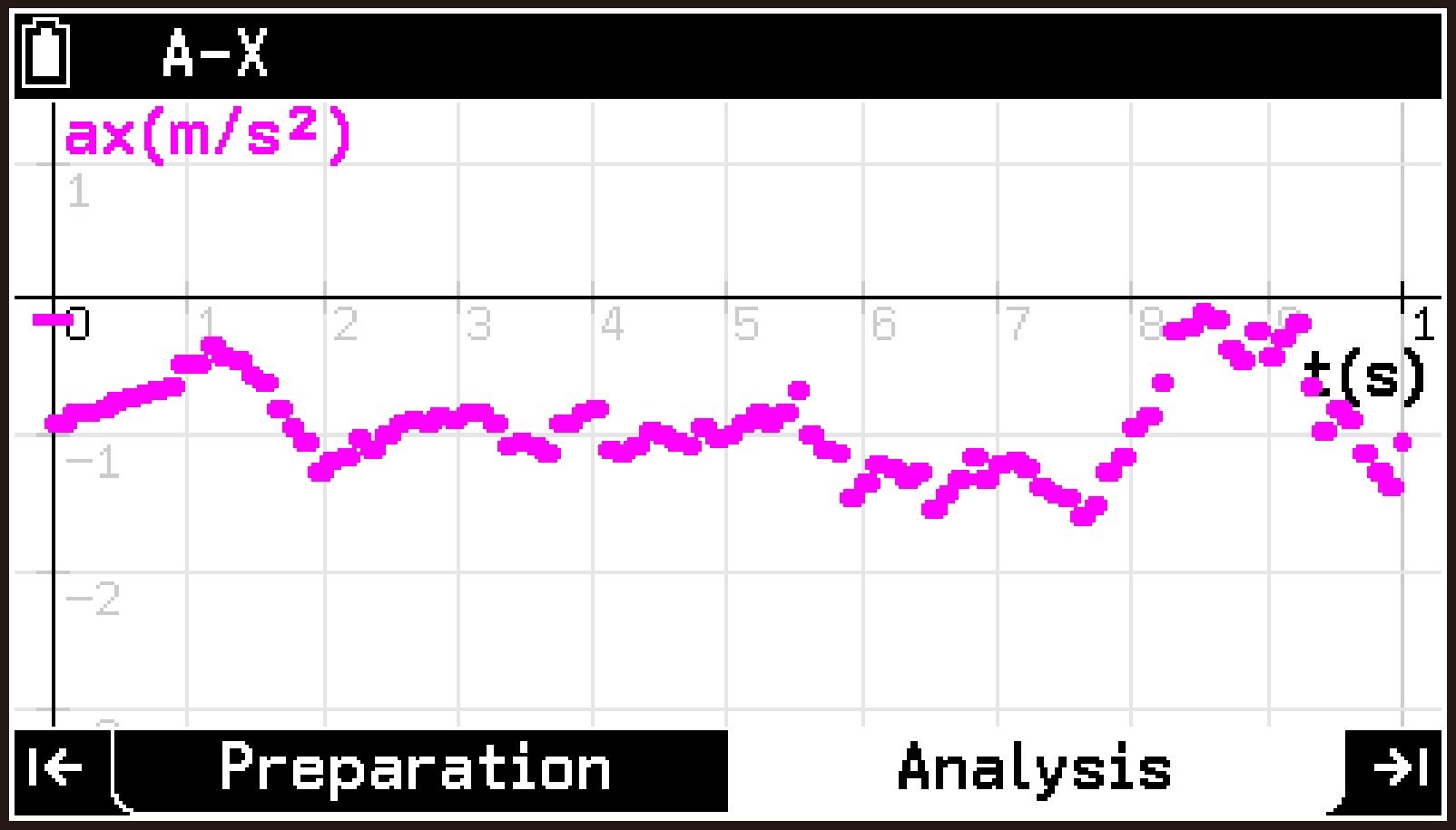
Press U or D to switch the graph display between A-X, A-Y, and A-Z.

Note
You can specify the point style, line style, and color to be used when drawing graphs. For details, see Specifying Line Style and Color for Graph Drawing.
Selecting a Sensor From the Library (CMA Sensors Only)
Some sensors may not be recognized automatically when connected to CLAB. In such cases, select the sensor from the library. This section explains how to use the library to select a sensor and assign it to CH3 of the E-CON5 app when a sensor connected to CLAB sensor terminal 3 is not recognized automatically.
-
Connect the calculator and CLAB, and then start the E-CON5 app.
-
Connect the sensor you want to use to CLAB sensor terminal 3.
-
Use d and u to highlight the CH3 row, and then select T > [Sensor Menu] > [Library].
-
Use d and u to highlight the sensor you want to assign to CH3, and then press O.
This displays the E-CON5 app top screen.
If the display contents of the top screen do not change, it means the sensor was not recognized automatically.
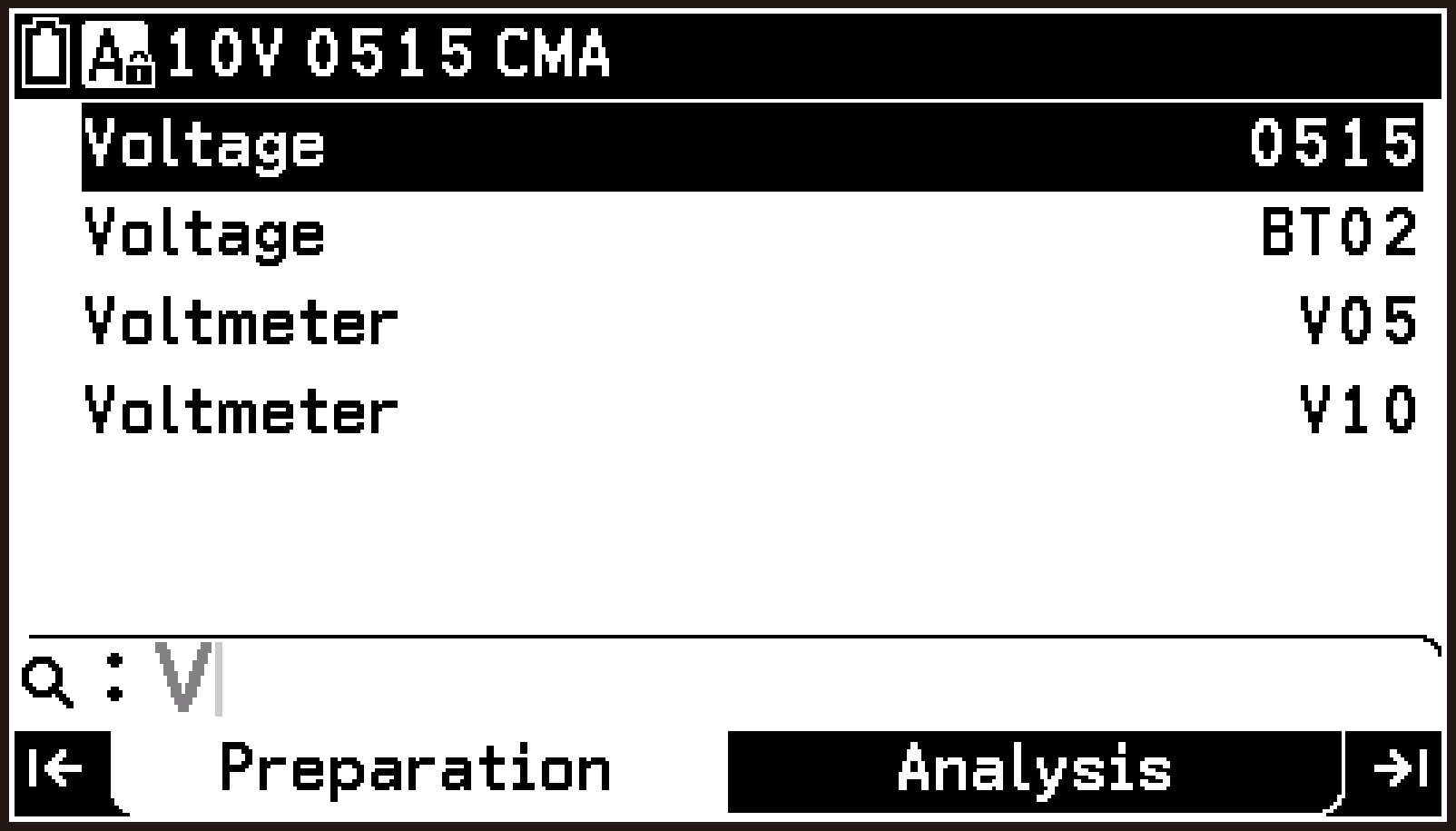
This switches to the library screen, which shows a list of CMA sensors in alphabetical order.
On this screen, you can enter characters to filter the list to sensors whose names begin with the entered string. For example, entering “V” lists only sensors whose names begin with “V”.
This returns to the top screen. The CH3 row now shows measured values based on signals from the connected sensor.
The icon on the left end of the CH3 row changes from ![]() to
to ![]() . For details about the meaning of this icon, see Top Screen Display Contents.
. For details about the meaning of this icon, see Top Screen Display Contents.
To remove the assignment of a sensor selected from the library
Highlight the channel (CH1, CH2, or CH3) that has a library sensor assigned, and then select T > [Sensor Menu] > [Remove Sensor].
Note
If necessary, you can change the measurement range and display unit of the sensor. For details, see Changing the Measurement Range and Display Unit of a Sensor.
To use a sensor that is not recognized automatically and is not in the library, see Creating a Custom Sensor (Preparation Tab).
Displaying Sensor Information for All Channels
-
Highlight the first row of the top screen and press O.
-
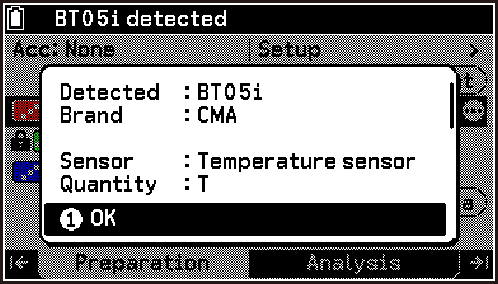
On the Setup menu that appears, select [Sensor Information].
This displays the following sensor information dialog.
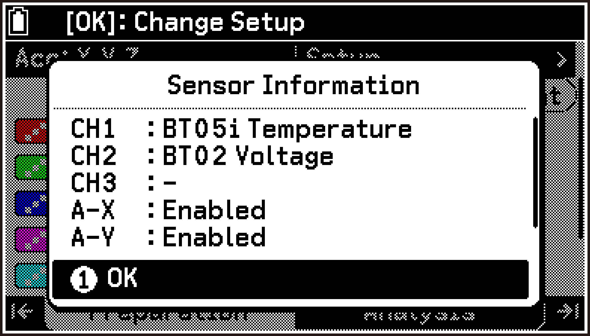
The information displayed in this dialog is as shown below.
|
Item |
Displayed Information |
|---|---|
|
CH1, CH2, CH3 |
Shows the model number and name of sensors recognized automatically or selected from the library. Shows “Custom” for a channel assigned a custom sensor. |
|
A-X, A-Y, A-Z |
Shows whether the CLAB built-in accelerometer is enabled (Enabled) or disabled (Disabled) for the -axis, -axis, and -axis. |
Displaying CLAB Version Information
-
Highlight the first row of the top screen and press O.
-
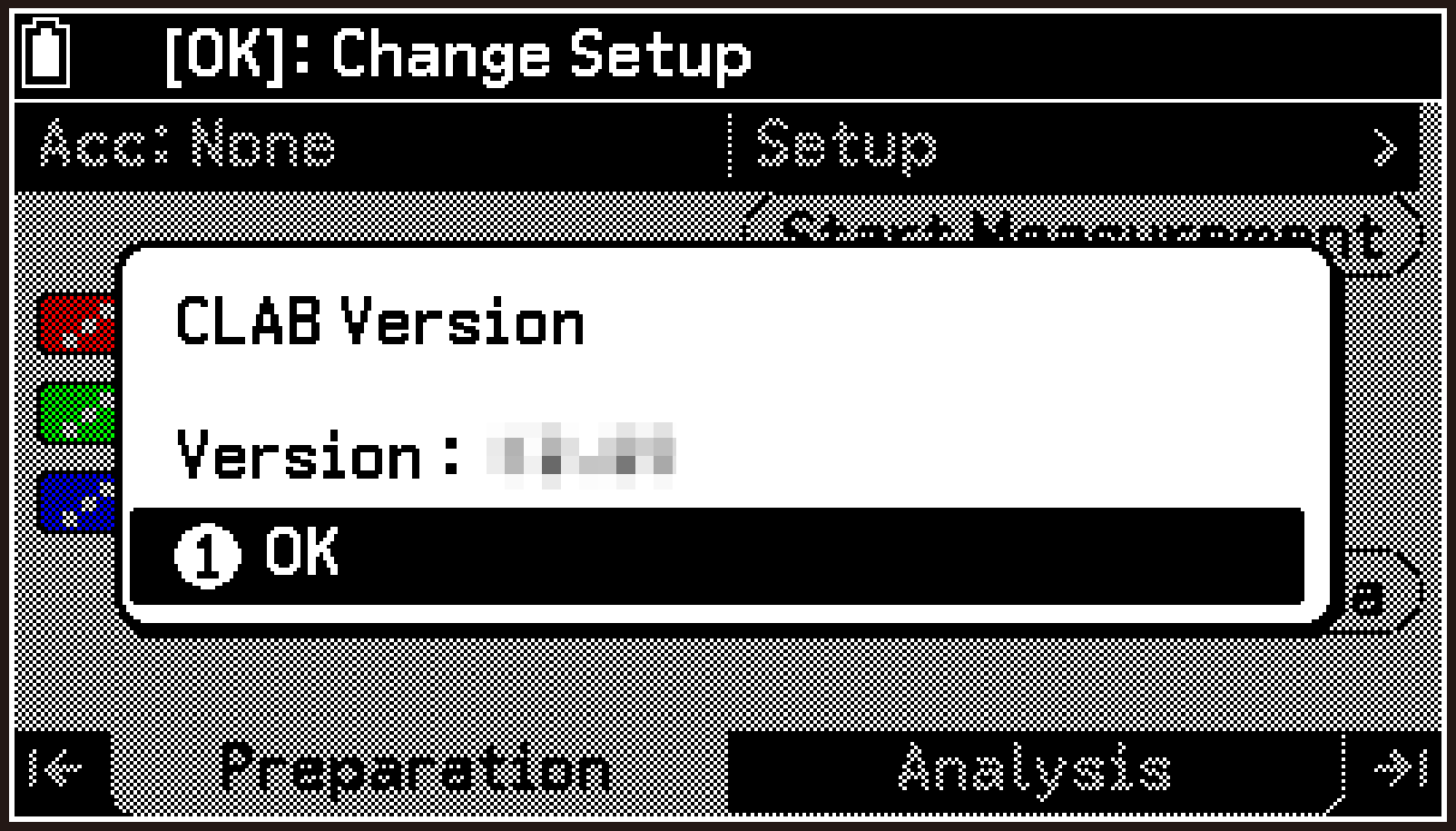
On the Setup menu that appears, select [CLAB Version].
This displays the CLAB version information dialog.
Saving and Recalling Setups
You can save the current E-CON5 app setup as a file and recall it later for use.
Note
For details about the settings saved in a setup and about various setup operations, see Using Setup Memory (Preparation Tab).
To save a setup
-
Configure sensor, measurement method, and graph drawing settings according to the measurement you want to perform.
-
Highlight the first row of the top screen and press O.
-
On the Setup menu that appears, select [Setup Memory].
-
Highlight the first row of the file list screen, and then press O.
-
On the menu that appears, select [Save Current Setup].
-
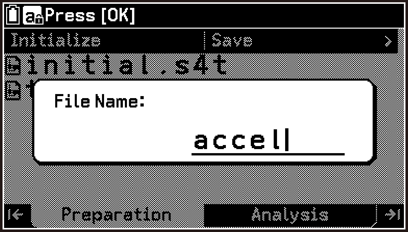
Enter a filename of up to eight characters, and then press O.
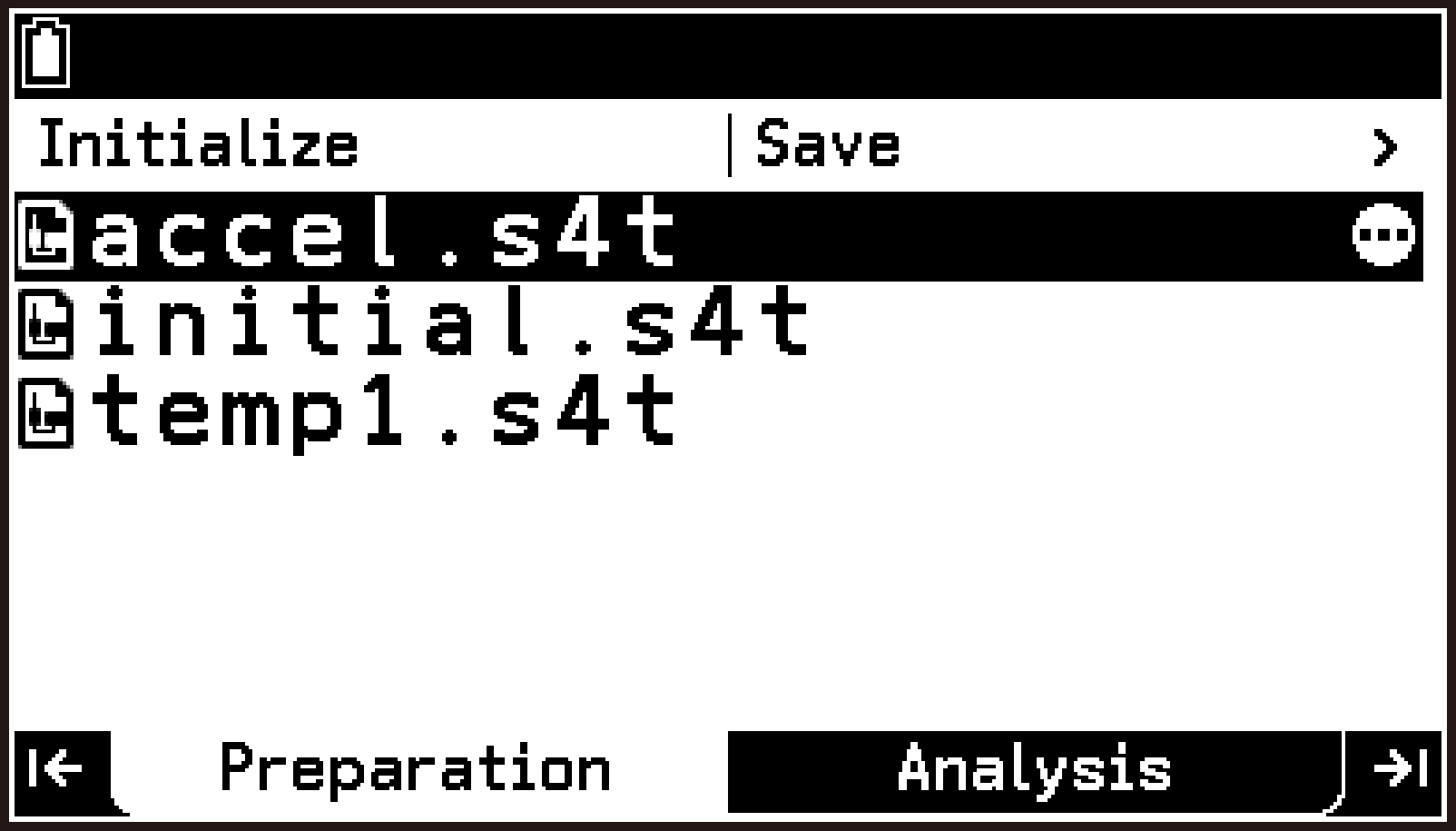
This displays the setup file list screen.
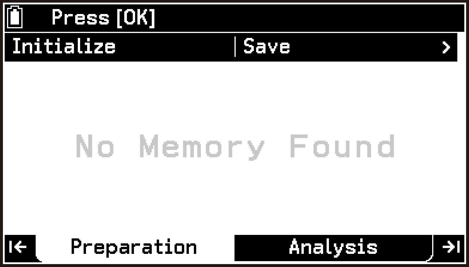
No setups saved
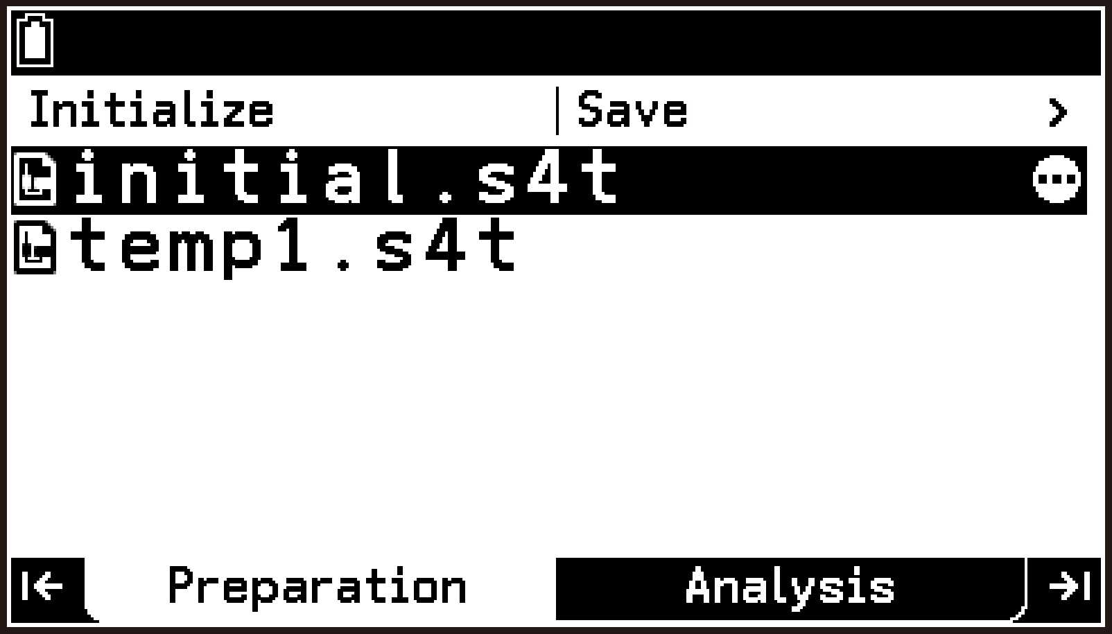
Setups already saved
This displays the filename input dialog.
This saves the current setup as a file.
To recall a setup
-
Perform steps 2 and 3 of the procedure under To save a setup to display the setup file list screen.
-
Use d and u to highlight the file whose setup you want to recall.
-
Select T > [Open Memory].
-
To recall the setup, select [OK] on the confirmation dialog.
-
To return to the top screen, press b.
This displays the “Clear current setup?” confirmation dialog.
This returns to the file list screen. (The screen appearance after recalling is the same as that before recalling.)
You can now start measurement using the recalled setup.
If information for an automatically recognized sensor is recalled from a setup, the sensor model number appears in red (as in the CH1 row on the screen to the right) while the sensor is not connected. Make sure you have the correct sensor connected before starting measurement.

Top Screen Display and Menus (Preparation Tab)
Top Screen Display Contents
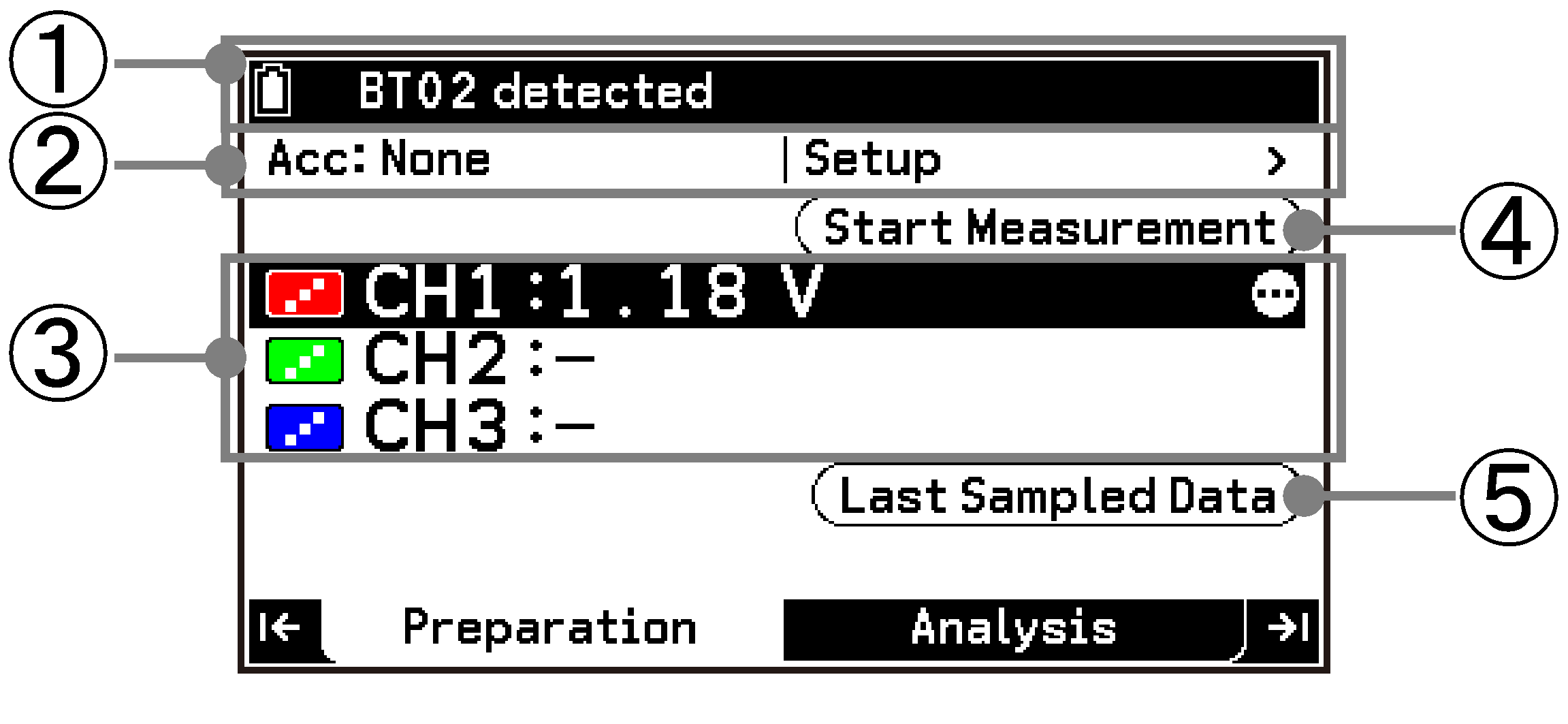
The first screen that appears when you start the E-CON5 app is the top screen. The contents of the top screen are shown below.
Acceleration disabled
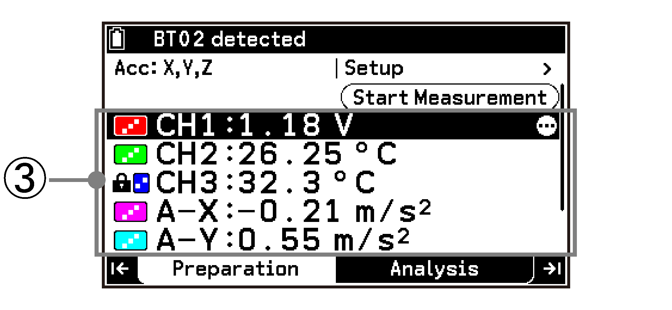
-axis, -axis, and -axis accelerometers enabled
-
The status bar shows information and explanations for the row or button currently highlighted on the top screen.
-
“Acc” at the left end of this row shows the enabled/disabled status of each axis of the accelerometer. When all axes are disabled, “None” is shown. When the -axis, -axis, or -axis is enabled, the letter representing the enabled axis (X, Y, or Z) is displayed.
Highlighting this row and pressing O displays the Setup menu. For details about the items on the menu, see Top Screen Setup Menu. -
These rows show the measured values from sensors connected to CH1, CH2, and CH3, and from enabled accelerometer axes. The icons on the left end of each row indicate the drawing style and color*1 for graph drawing, as well as the sensor configuration status.
-
Highlighting this button and pressing O starts measurement using the current setup.
-
Highlighting this button and pressing O displays the graph screen (Analysis tab). You can also display the graph screen by pressing < or >.
![]() … Indicates a sensor recognized automatically. This indication is also shown when no sensor is connected.
… Indicates a sensor recognized automatically. This indication is also shown when no sensor is connected.
![]() … Indicates a manually specified sensor.*2
… Indicates a manually specified sensor.*2
For details, see Specifying Line Style and Color for Graph Drawing.
Applies when you specify a sensor using one of the following methods:
Sensor specified using T > [Sensor Menu] > [Library]. See Selecting a Sensor From the Library (CMA Sensors Only).
Custom sensor created using T > [Sensor Menu] > [Custom Sensor]. See Creating a Custom Sensor (Preparation Tab).
When a sensor recognized automatically is recalled from setup memory. See Saving and Recalling Setups.
Top Screen Setup Menu
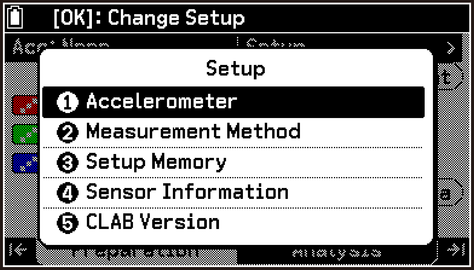
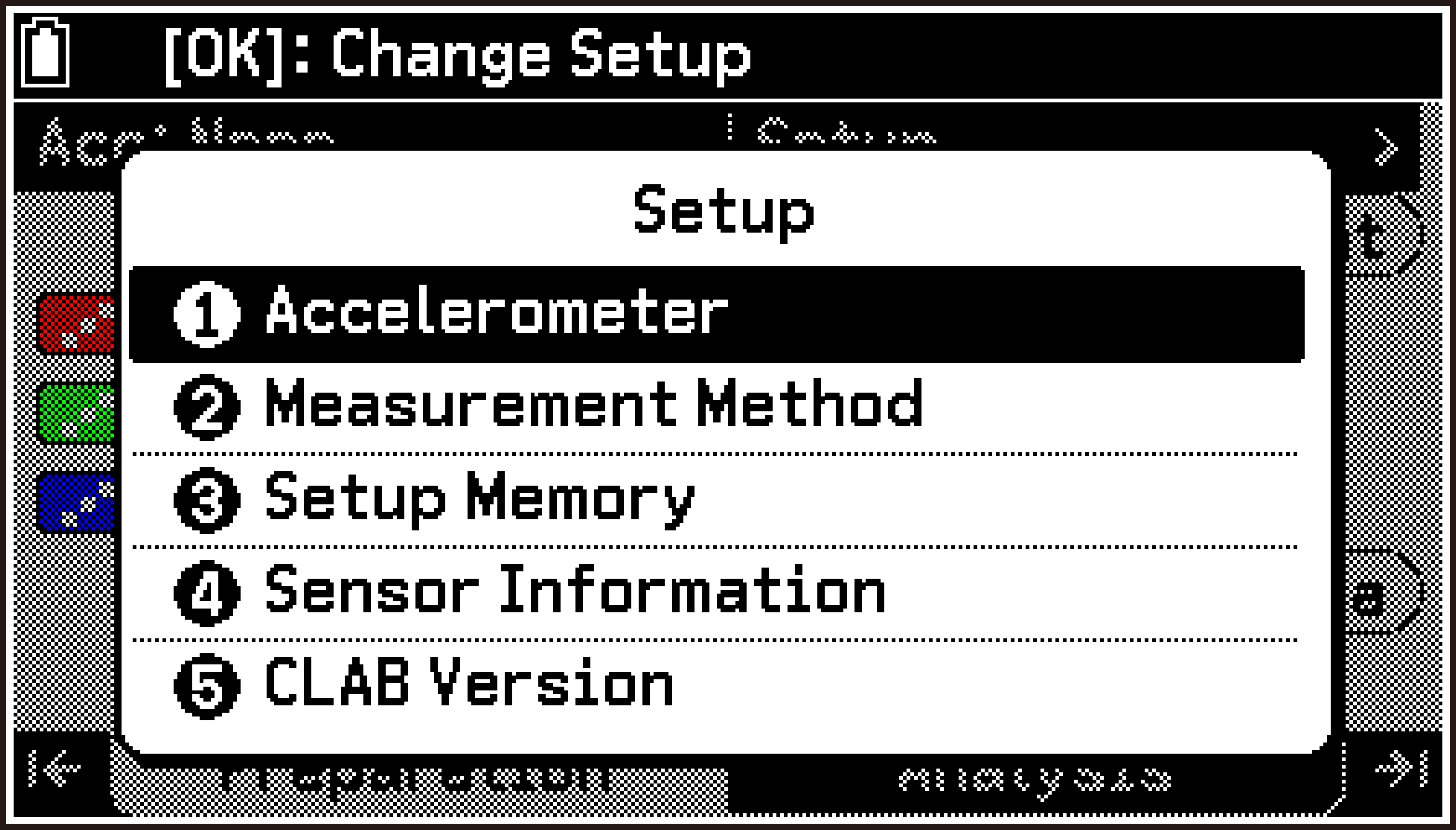
Highlighting the first row of the top screen and then pressing O displays the following Setup menu.
|
For information about this menu Item: |
Go here: |
|---|---|
|
[Accelerometer] |
|
|
[Measurement Method] |
|
|
[Setup Memory] |
|
|
[Sensor Information] |
|
|
[CLAB Version] |
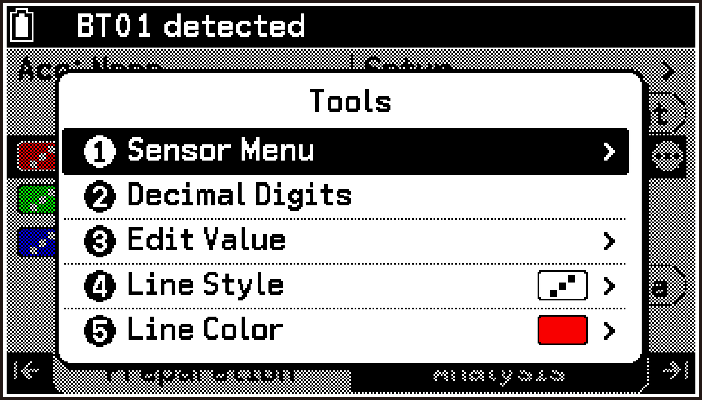
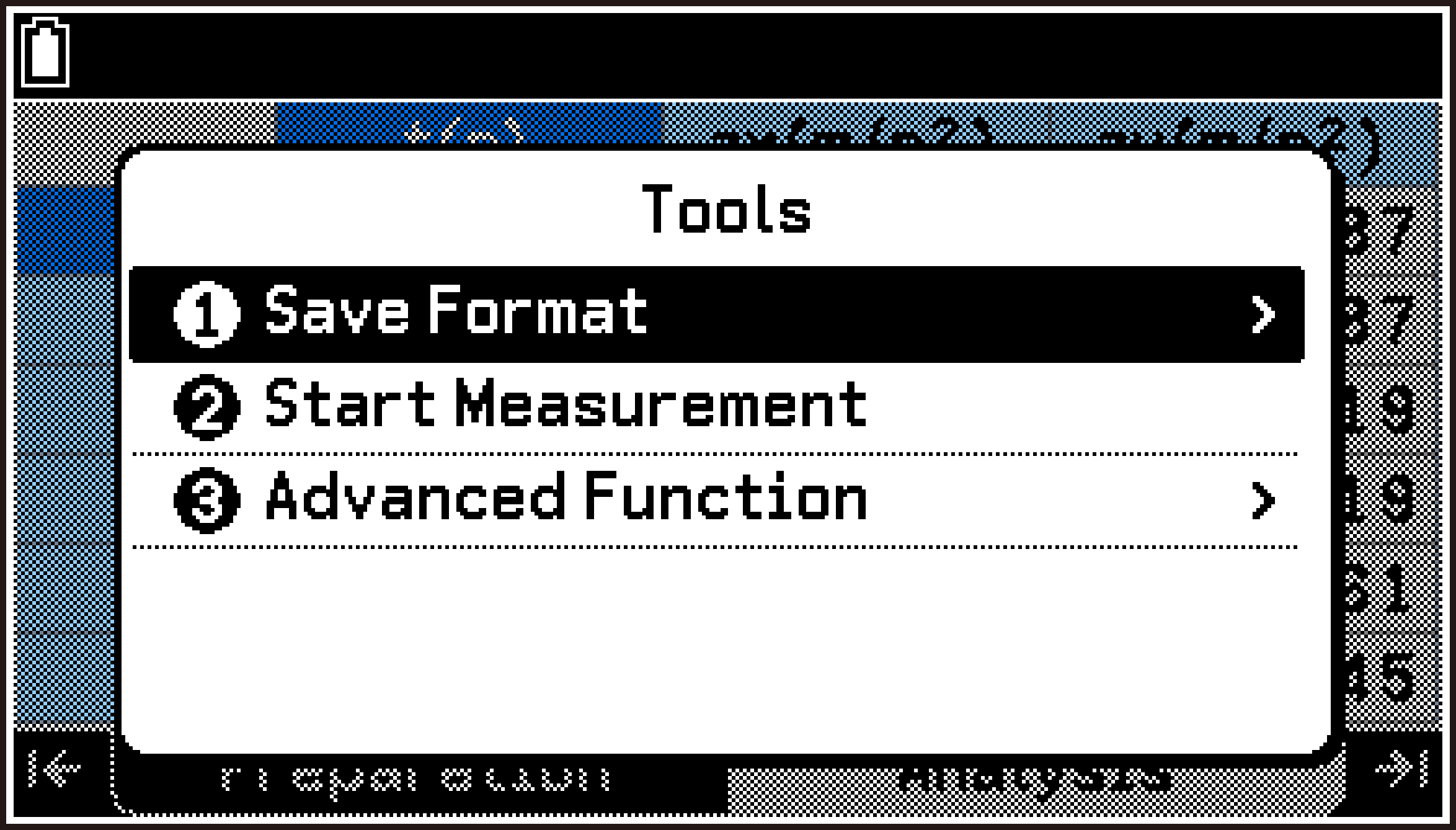
Top Screen Tools Menu
Highlighting one of the rows (CH1, CH2, CH3, A-X, A-Y, A-Z) on the top screen and then pressing T displays the Tools menu for changing settings or displaying information for the selected channel.
|
For information about this menu Item: |
Go here: |
|
|---|---|---|
|
T > [Sensor Menu] > |
[Library] |
|
|
|
[Custom Sensor] |
|
|
|
[Select Range] |
|
|
|
[Information] |
|
|
|
[Remove Sensor] |
To remove the assignment of a sensor selected from the library |
|
T > [Decimal Digits] |
Specifying the Number of Decimal Places for Displayed Values |
|
|
T > [Edit Value] > |
[New Value] |
|
|
T > [Line Style] |
||
|
T > [Line Color] |
||
Specifying the Measurement Method (Preparation Tab)
Use the following procedure to specify the measurement method.
-
Highlight the first row of the top screen and press O.
-
On the Setup menu that appears, select [Measurement Method].
-
Highlight CLAB, and then press O. Use the menu that appears to select the CLAB operating mode (Connected or Standalone).
-
Highlight Type, and then press O. Use the menu that appears to select the measurement type (Time-based, Manual or Interval).
-
Change the settings of the remaining items according to the measurement type.
-
To complete the setting procedure and return to the top screen, press b.
This displays the Measurement Method screen.
For details, see CLAB Operating Modes.
If you selected Connected in step 3, the measurement type is fixed to Time-based.
For details about each measurement type, see Measurement Types.
For details, see Time-based Type Setting Items, Manual Type Setting Items, and Interval Type Setting Items.
The following describes each item on the Measurement Method screen.
CLAB Operating Modes
CLAB has the following two operating modes.
Connected Mode
This is the operating mode when you select CLAB: Connected on the Measurement Method screen. Connected mode is the initial default setting for the E-CON5 app.
In Connected mode, measurement is performed while the calculator and CLAB remain connected. During measurement, CLAB is controlled by the E-CON5 app. This mode provides three measurement types: Time-based, Manual, and Interval. For details, see Measurement Types. When using the Time-based type with a relatively low sampling frequency, or when using the Manual type or Interval type, the E-CON5 app shows measurement data in real time so you can observe progress during measurement.
In this mode, measurement data is saved in the calculator’s memory* and not in CLAB’s memory.
Standalone Mode
This is the operating mode when you select CLAB: Standalone on the Measurement Method screen.
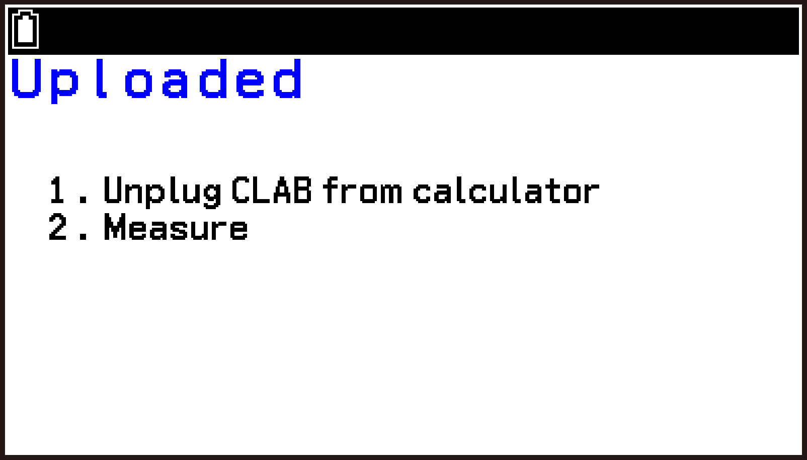
In Standalone mode, you first upload the measurement setup from the calculator’s E-CON5 app to CLAB. Before starting measurement, disconnect the cable between the calculator and CLAB, and then perform measurement using CLAB alone.
This method is convenient, for example, when you want to collect data outdoors over an extended period.
In this mode, measurement data is saved temporarily in CLAB’s memory. After measurement is complete, you can download the data from CLAB to the calculator’s memory.*
For details, see E-CON5 App Data Storage.
Measurement Types
CLAB has three measurement types.
Time-based Type
This is the measurement type when you select Type: Time-based on the Measurement Method screen.
With this type, measurement data from sensors is collected for a specified length of time at a specified sampling frequency. Measurement ends automatically when the specified time elapses.
For details about the setting items when this type is selected, see Time-based Type Setting Items.
Manual Type
This is the measurement type when you select Type: Manual on the Measurement Method screen. This type is available only in Connected mode.
With this type, you specify in advance the number of times (number of samples) that data will be measured. After measurement starts, measurement data from the sensors is collected each time you press O. In addition to sensor measurement data, you can also collect data entered manually at the same time. For example, you can use this function to verify Boyle’s law in an experiment: measuring gas pressure using a pressure sensor and manually entering the corresponding volume value measured separately. Measurement ends when the specified number of samples has been collected.
For details about the setting items when this type is selected, see Manual Type Setting Items.
Interval Type
This is the measurement type when you select Type: Interval on the Measurement Method screen. This type is available only in Connected mode.
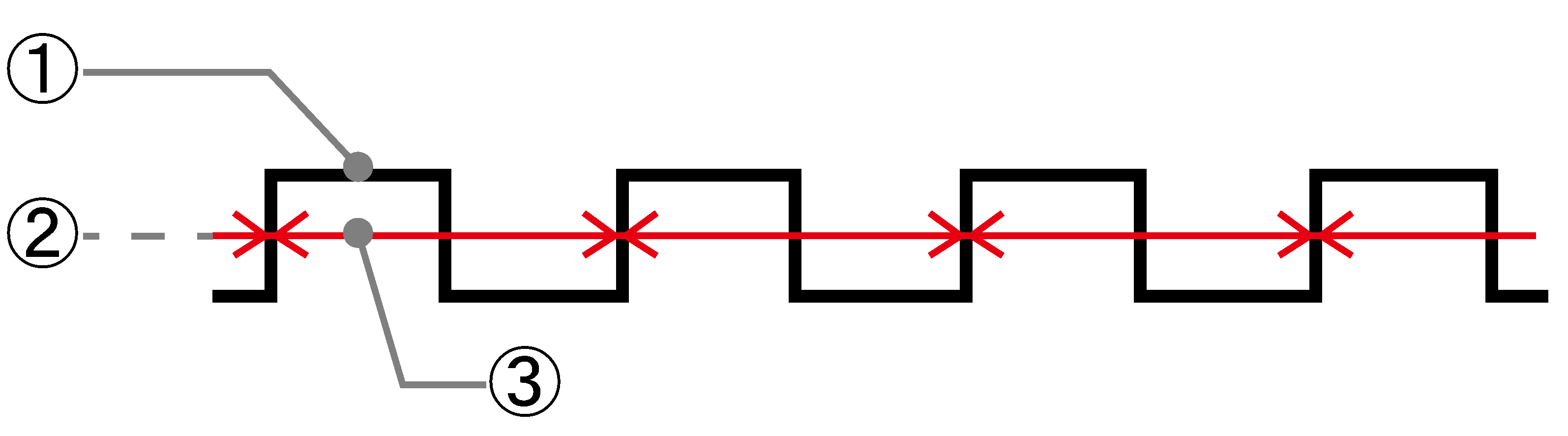
With this type, the measurement data collected is the time interval between two points at which the measurement value from the specified channel (CH1, CH2, or CH3) crosses a specified threshold value (exceeds it [Rise] or falls below it [Fall]).
For example, with the initial default Rise-Rise setting, the time interval indicated by ↔ in the figure below is collected as measurement data.
-
Measurement value from sensor
-
Threshold value
-
Time interval
For details about the setting items when this type is selected, see Interval Type Setting Items.
Time-based Type Setting Items
The items and their functions when you select Type: Time-based on the Measurement Method screen are described below.
In the explanations, options and values marked with “◆” are initial defaults.
Unit
Specifies the unit for Duration and Frequency. Available options:
Duration unit: msec (milliseconds), sec◆ (seconds), min (minutes), hour (hours)
Frequency unit: /msec (per a millisecond), /sec◆ (per a second), /min (per a minute), /hour (per an hour)
If you change the Unit setting of either the Duration or the Frequency item, the value of that item is recalculated according to the new unit. For example, if Duration is currently 10 (sec) and you change the Unit from sec to msec, the Duration value becomes 10,000 (msec).
Duration
Specifies the measurement time (Initial Default: 10 seconds). If you change the Duration value, the Samples value is automatically adjusted according to the current Frequency value and the new Duration value.
Frequency
Specifies the sampling frequency, which is the number of measurements per unit of time (Initial Default: Once/second). If you change the Frequency value, the Samples value is automatically adjusted according to the current Duration value and the new Frequency value.
Samples
Specifies the number of samples, which is the number of measurements within the entire measurement time (Initial Default: 11). If you change the Samples value, the Duration value is automatically adjusted according to the current Frequency value and the new Samples value.
Trigger
Specifies the measurement start condition. The available options depend on the operating mode.
CLAB in Connected mode
None◆: Measurement starts when you select Start Measurement (button or menu) with the E-CON5 app.
CH1, CH2, CH3: Measurement starts when the measured value from the selected channel (CH1, CH2, or CH3) goes above or below a specified value. Use the Level and Direction items to specify the measurement value and the trigger timing. When you select this setting, the E-CON5 app displays the following standby screen after you choose Start Measurement (button or menu).
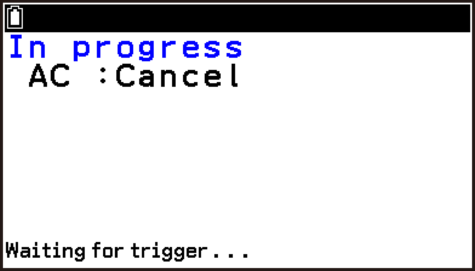
[OK]: When you select this setting, the E-CON5 app shows the following standby screen after you choose Start Measurement (button or menu). Pressing O while this screen is displayed starts measurement.

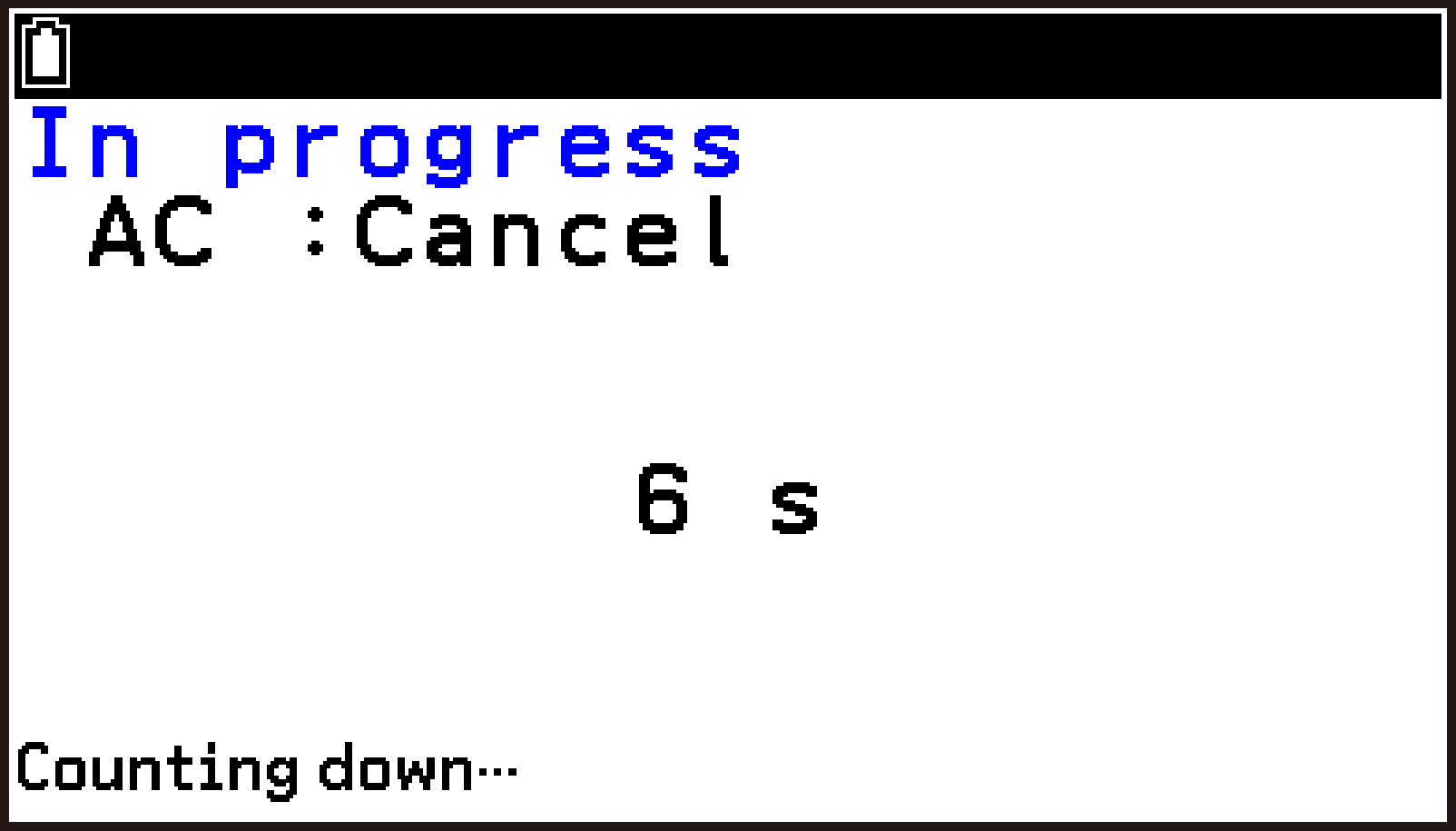
Countdown: When you select this setting, the E-CON5 app displays the following countdown screen after you choose Start Measurement (button or menu). Measurement starts automatically after the specified countdown time elapses. Use the Countdown item to specify the countdown duration.
CLAB in Standalone mode
CLAB button◆: When you select this setting, the E-CON5 app shows the following screen after you choose Start Measurement (button or menu). After disconnecting the cable between the calculator and CLAB, press the CLAB power button to start measurement.

CH1, CH2, CH3: When you select this setting, the E-CON5 app displays the following screen after you choose Start Measurement (button or menu).
After disconnecting the cable between the calculator and CLAB, measurement starts when the measured value from the selected channel (CH1, CH2, or CH3) goes above or below a specified value. Use the Level and Direction items to specify the measurement value and the trigger timing.
Even with this setting, you can press the CLAB power button to forcibly start measurement.
Level
This setting is displayed when you select CH1, CH2, or CH3 for Trigger. Use it to specify a measurement start value. Display of the unit of the measurement value is fixed according to the sensor currently connected to the channel you selected for Trigger.
Direction
This setting is displayed when you select CH1, CH2, or CH3 for Trigger. Use it to specify when measurement starts relative to a set value. The available options are:
Up: Starts measurement when the sensor value rises above the value specified by Level.
Down: Starts measurement when the sensor value falls below the value specified by Level.
Both◆: Starts measurement when the sensor value either rises above or falls below the value specified by Level.
Countdown
This setting appears when you select Countdown for Trigger. Use it to specify the number of seconds before measurement starts.
You can specify a value from 1 to 3,599 seconds (default: 10 seconds).
Manual Type Setting Items
When you select Type: Manual on the Measurement Method screen, you can specify the setting items described below.
In the explanations, options and values marked with “◆” are initial defaults.
Samples
Specifies the number of samples. (Initial Default: 10)
Input
Specifies whether only sensor measurements will be collected or data will be input manually. The available options are:
None◆: No manual data entry. Collect only sensor measurements.
1 Entry, 2 Entries, 3 Entries: Specify how many values are to be entered manually with each measurement. You can also configure Quantity, Unit, and Digits settings for the number of manual entries you specify.
Quantity (Quantity1, Quantity2, Quantity3)
Enter up to eight characters or symbols* to indicate what the value represents (quantity symbol). For example, if the value represents temperature, enter “T” (the first letter of Temperature). If left blank, the initial defaults are q1, q2, q3.
Unit (Unit1, Unit2, Unit3)
Enter up to eight characters or symbols* to indicate the unit of the value. For example, if the value represents temperature in Celsius, enter “°C”. If left blank, the initial defaults are u1, u2, u3.
Digits (Digits1, Digits2, Digits3)
Specifies the number of decimal places for manually entered values. You can specify a value from 0 to 7 (Initial Default: 2). Manually entered values are rounded to the number of decimal places you specify. For example, if you specify 1 and enter 1.24, the stored data becomes 1.2. If you enter 1.25, the stored data becomes 1.3.
The characters you enter for Quantity and Unit are displayed on the manual input dialog, as the Y-axis label on the graph screen, and as the header on the table screen. The following shows how screens appear if you leave the initial default setting unchanged.
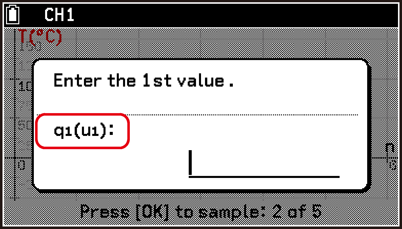
Input Dialog
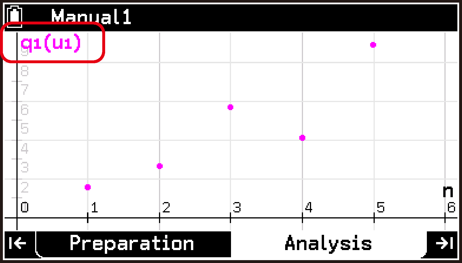
Graph Screen
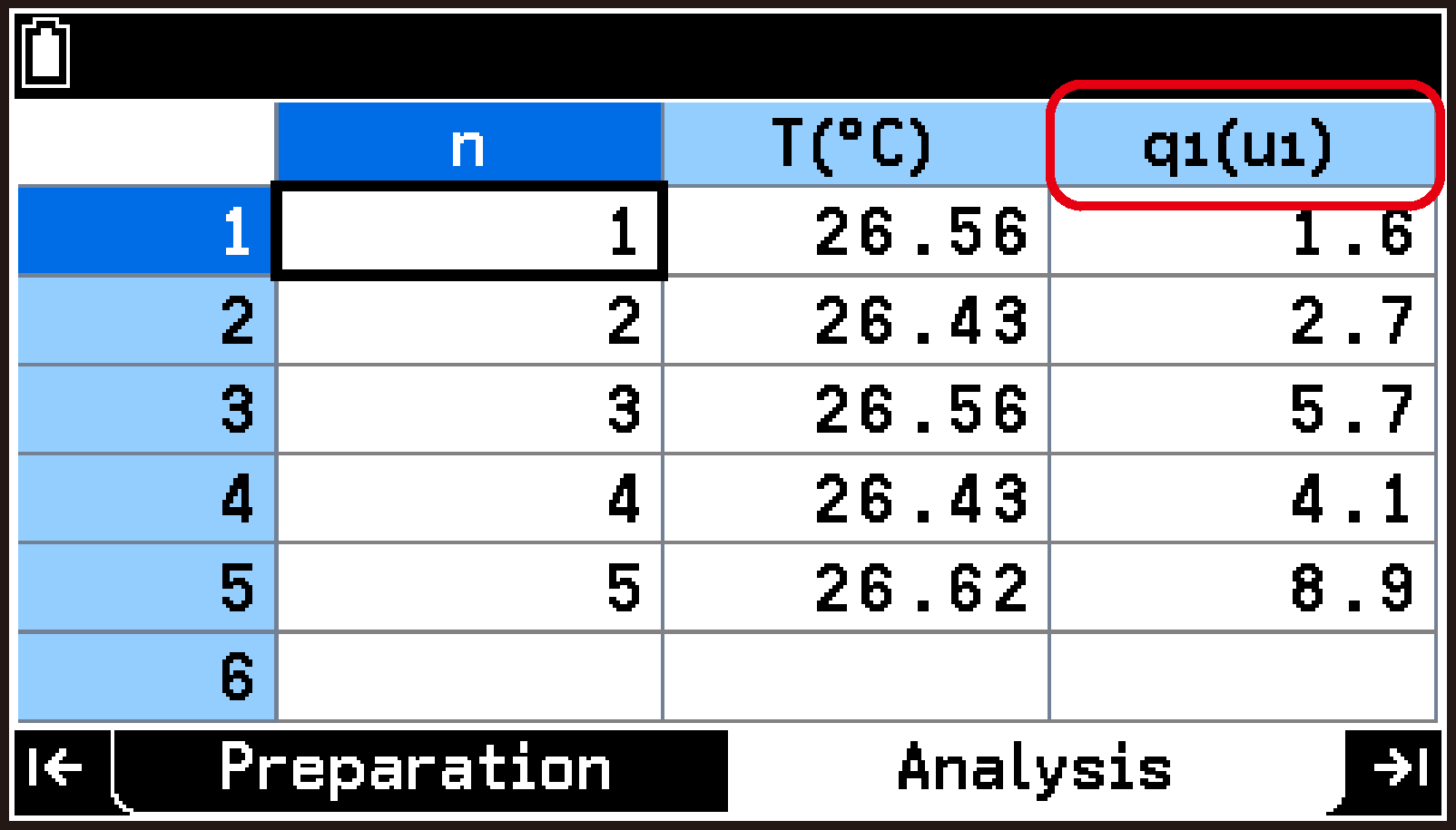
Table Screen
Interval Type Setting Items
When you select Type: Interval on the Measurement Method screen, you can specify the setting items described below.
In the explanations, options and values marked with “◆” are initial defaults.
Samples
Specifies the number of samples. (Initial Default: 10)
Source
Specifies the channel (CH1, CH2, CH3) to which the sensor used as the signal source is connected. This item is displayed in red as “None” in the following cases.
No sensor connected to the CLAB.
A sensor is connected to the CLAB, but no appropriate measurement range has been selected.
Threshold
Specifies the signal threshold. This value is used as the reference for determining the start and end points of the time intervals collected as data. The initial default value is 50% of the measurement range of the sensor being used as the signal source. For the relationship between the threshold and the collected time intervals, see Flank.
Flank
Defines “Rise” as the point where the sensor signal increases and crosses the Threshold value, and “Fall” as the point where it decreases and crosses the Threshold value. This setting provides the following options to specify which time intervals are collected as measurement data. In each case, the ↔ interval in the figure is collected as data.
|
Rise-Rise◆: Specifies collection of time intervals from Rise to Rise. |
 |
|
Fall-Fall: Specifies collection of time intervals from Fall to Fall. |
 |
|
Rise-Fall: Specifies collection of time intervals from Rise to Fall. |
 |
|
Fall-Rise: Specifies collection of time intervals from Fall to Rise. |
 |
|
Both: Specifies collection of both intervals from Rise to Fall and from Fall to Rise. |
 |
Repeat
By default, measurement ends automatically after the number of samples specified by Samples is collected. You can also configure this setting so that a confirmation dialog is displayed when the specified number of samples has been collected.
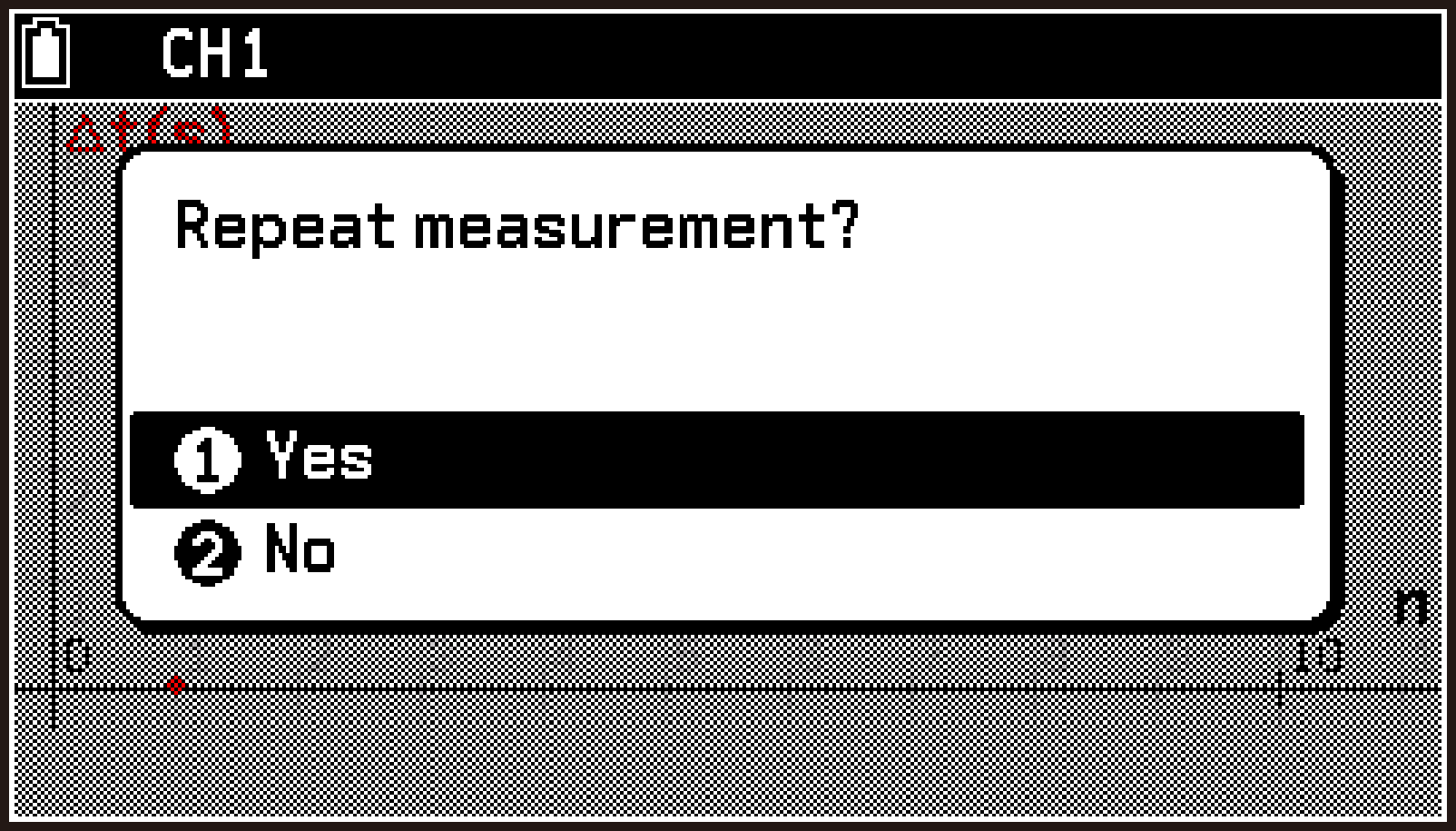
Off◆: Measurement ends automatically when the number of samples specified by Samples is collected.
On: Displays a confirmation dialog when the number of samples specified by Samples is collected.
Select [Yes] on the dialog to continue measurement until the same number of samples specified by Samples is collected again. The newly collected data is added after the previously collected data. Select [No] to end measurement.
Using Setup Memory (Preparation Tab)
A set of setup data stored in the E-CON5 app setup memory is called a setup. A setup includes all of the following setting information:
Sensor assignment to CH1, CH2, and CH3, and the enable/disable status of each axis of the accelerometer (all the settings displayed on the sensor details dialog)
Measurement method settings (all the settings displayed on the Measurement Method screen)
Graph drawing settings (all the settings displayed on the Graph View screen)
Changing any of these settings causes setup memory contents to be updated accordingly.
You can save the setup currently stored in setup memory as a file, or load a saved file to reproduce a setup.
Saving and Recalling Setups
See To save a setup and To recall a setup.
Viewing the Information of a Saved Setup
-
Highlight the first row of the top screen and press O.
-
On the Setup menu that appears, select [Setup Memory].
-
Use d and u to highlight the file whose setup information you want to view.
-
Select T > [Information].
-
To close the dialog, press O.
This displays the setup file list screen.
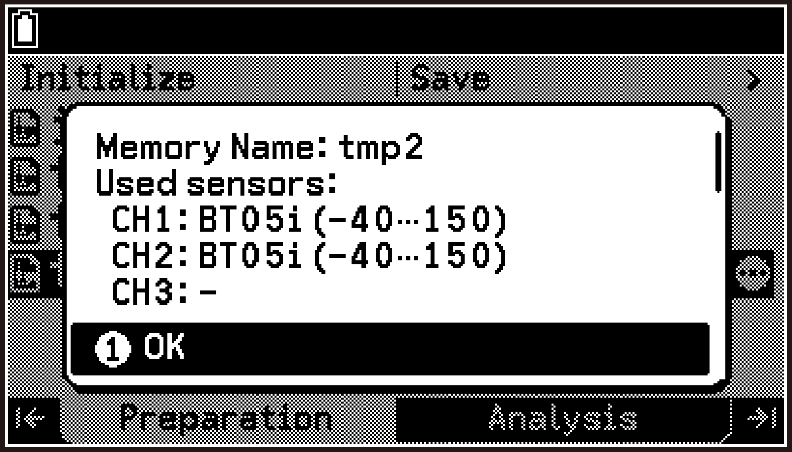
This displays the setup information dialog, which shows the following information:
Sensor assignment to CH1, CH2, and CH3
Enabled/disabled status of each accelerometer axis
Current measurement method settings
You can scroll the display using d or u.
Deleting a Saved Setup
-
Perform steps 1 and 2 of the procedure under Viewing the Information of a Saved Setup to display the setup file list screen.
-
Use d and u to highlight the file whose setup you want to delete.
-
Select T > [Delete Memory].
-
To delete, select [OK] on the confirmation dialog.
This displays the “Delete Memory?” confirmation dialog.
Initializing Setup Memory
The following operation deletes all setting information currently stored in setup memory and returns the E-CON5 app to its initial state.
-
Perform steps 1 and 2 of the procedure under Viewing the Information of a Saved Setup to display the setup file list screen.
-
Highlight the first row of the file list screen, and then press O.
-
On the menu that appears, select [Initialize Current Setup].
-
To initialize, select [OK] on the confirmation dialog.
This displays the “Clear current setup?” confirmation dialog.
Creating a Custom Sensor (Preparation Tab)
The Preparation tab lets you create a custom sensor and define its settings. By performing the calibration operation, you can also adjust the relationship between the input voltage values from the sensor and the measurement values displayed by the E-CON5 app.
Creating a New Custom Sensor
-
Connect the calculator and CLAB, and then start the E-CON5 app.
-
Highlight one of the channels (CH1, CH2, CH3). The channel you highlight should meet one of the following conditions.
-
Select T > [Sensor Menu] > [Custom Sensor].
-
Highlight “New Custom Sensor”, and then press O.
-
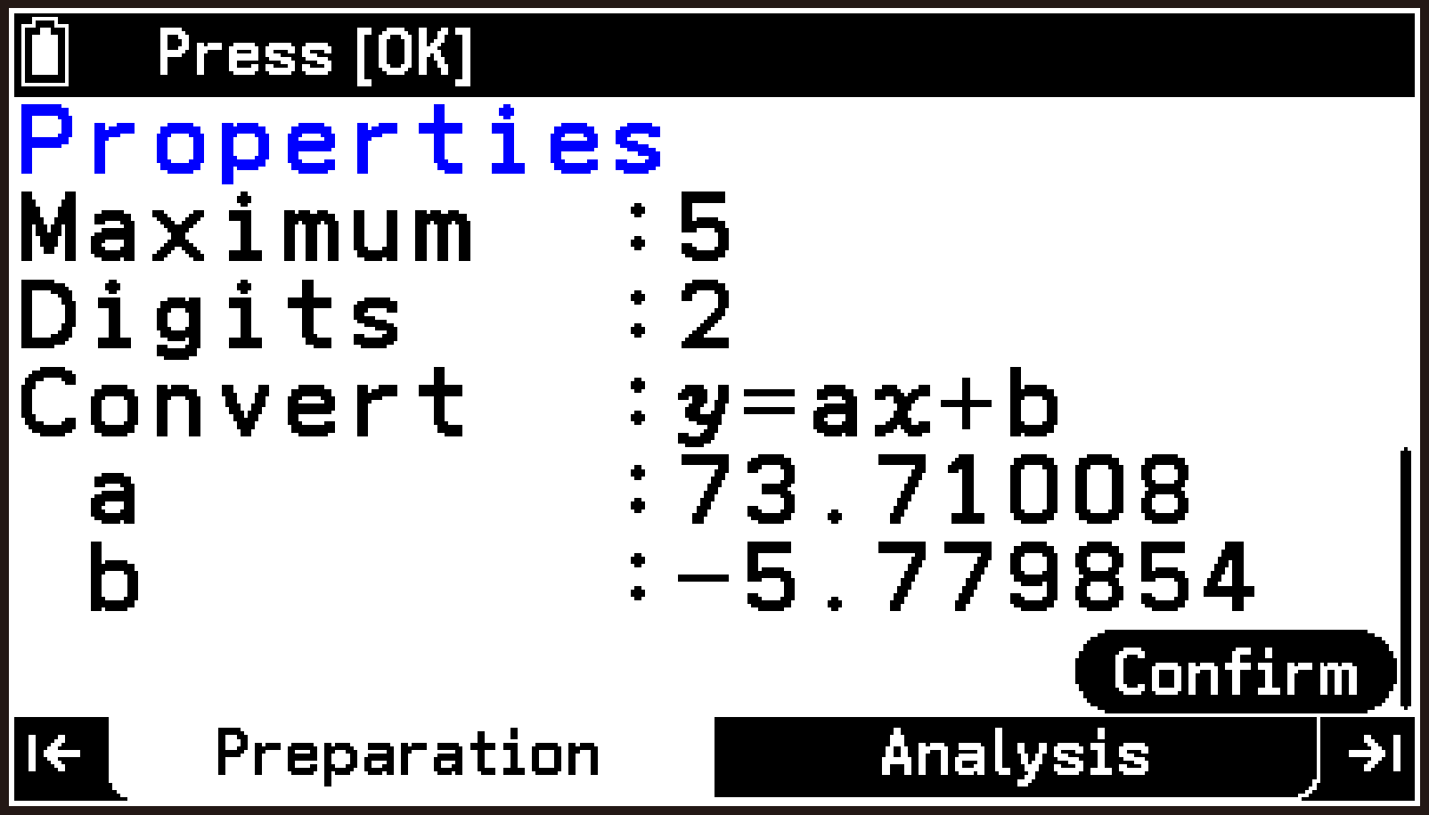
On the Properties screen, configure the settings of each item from Name through Convert.
-
Perform calibration.
-
After configuring all of the settings, highlight
 , and then press O.
 -
To return to the top screen, press b.
This displays the E-CON5 app top screen.
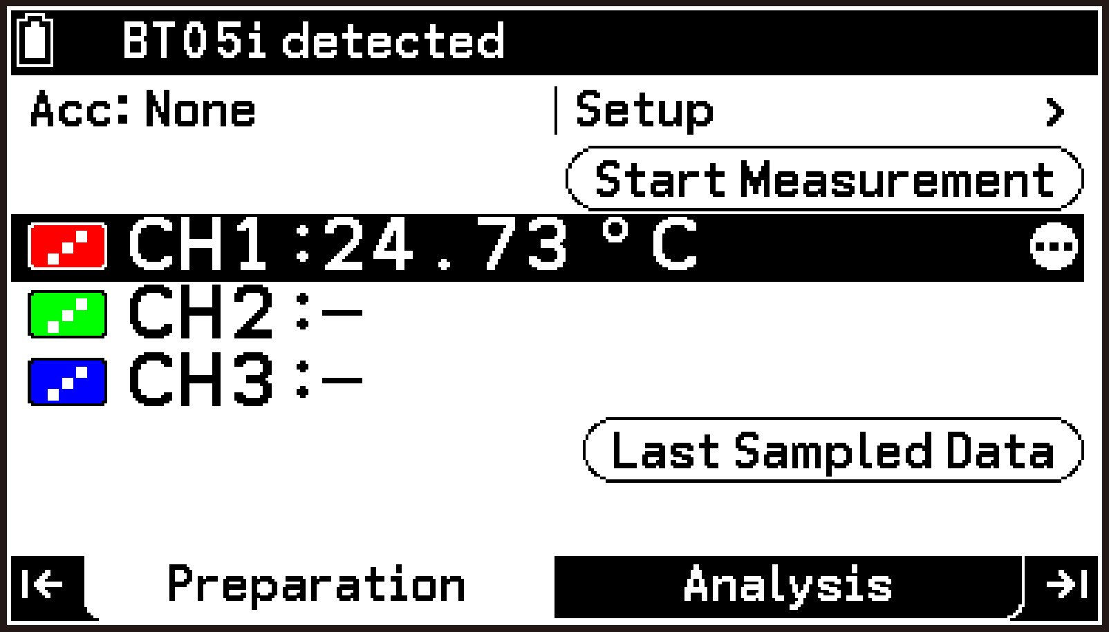
No sensor connected: A channel that shows “-”, such as CH2 and CH3 in the screen to the right.
Library sensor or custom sensor assigned: A channel that shows the ![]() icon to the left.
icon to the left.
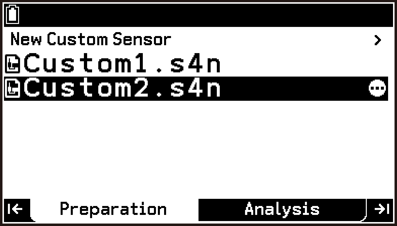
This displays the custom sensor file list screen.
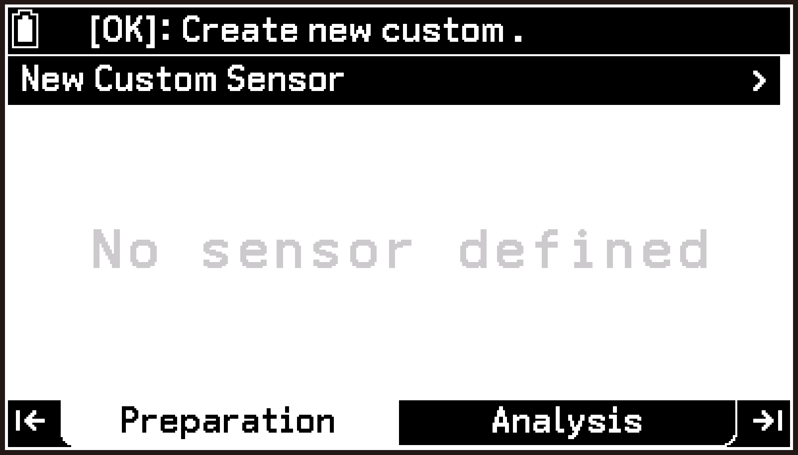
No custom sensor saved
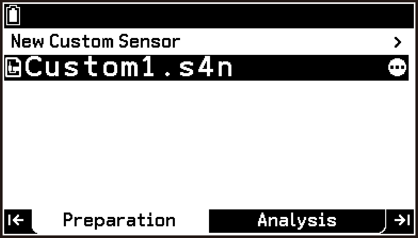
Custom sensor saved
This displays the Properties screen for creating a new custom sensor.
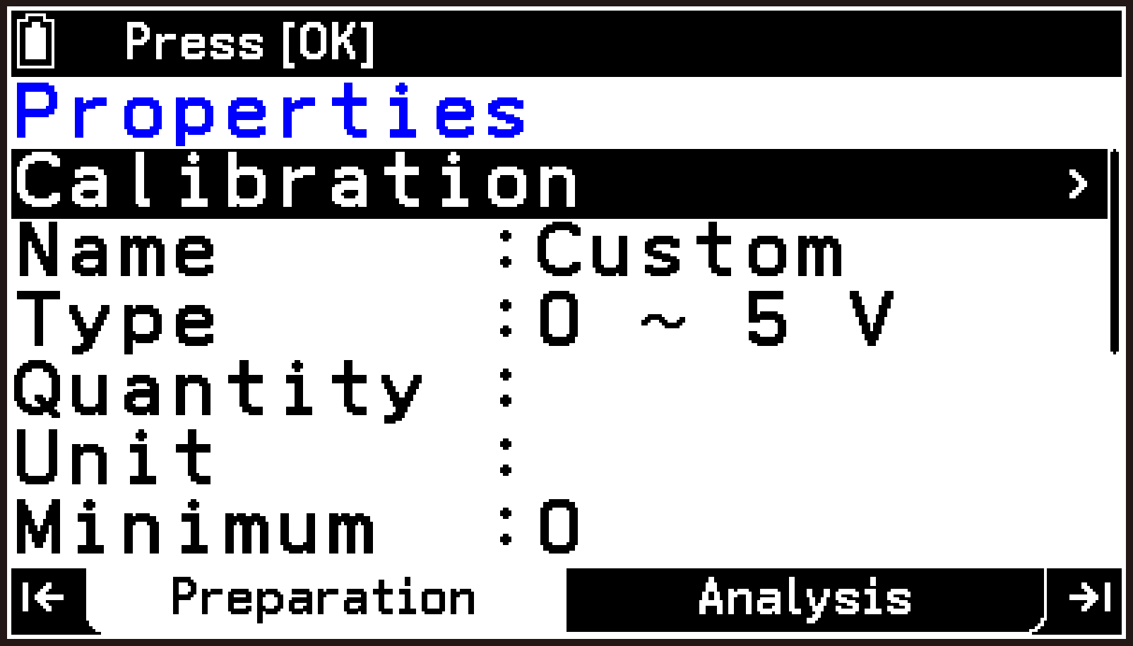
For details about these items, see Custom Sensor Setting Item Details.
For information about the calibration operation, see Performing Calibration.
This adds the newly created custom sensor to the file list screen.
Custom Sensor Setting Item Details
In the explanations, options and values marked with “◆” are initial defaults.
Calibration
Selecting this item displays the screen for performing calibration. For information about the calibration operation, see Performing Calibration.
Name
Highlight this item and then press O. On the dialog that appears, enter up to eight characters as the name of the custom sensor. The name you enter here is displayed on the custom sensor file list screen.
Type
Highlight this item and then press O. Use the menu that appears to select the sensor type. The following two sensor types are available.
0 ~ 5 V◆: Sensor with a voltage range of 0 V to 5 V
-10 ~ 10 V: Sensor with a voltage range of -10 V to 10 V
Quantity
Use the input dialog that appears when you highlight this item and press O to enter up to eight characters or symbols as the quantity symbol. The quantity symbol indicates what the sensor’s measured values represent. The initial default is blank.
Unit
Use the input dialog that appears when you highlight this item and press O to enter up to eight characters or symbols to indicate the unit of the sensor’s measured values. The initial default is blank.
Minimum
Specifies the minimum value displayed as the sensor measurement. You can enter a value from -500,000 to 500,000 (Initial Default: 0).
Maximum
Specifies the maximum value displayed as the sensor measurement. You can enter a value from -500,000 to 500,000 (Initial Default: 5).
Digits
Specifies the number of decimal places displayed for sensor measurements. You can enter an integer from 0 to 7 (Initial Default: 2). Displayed values are rounded to the number of decimal places you specify.
Convert
Highlight this item and then press O. Use the menu that appears to select the function to be used for sensor calibration. The functions below are available. The voltage value () from the sensor is converted by the selected function and displayed as the measurement value ().
◆: Linear function
: Quadratic function
: Logarithmic function
Depending on the function you select, enter the required coefficient values (a, b, c) in the rows displayed below Convert. You can enter values in the range of -1,000,000 to 1,000,000. You can enter coefficient values manually, but normally you select a function first, and then perform calibration using the following procedure.
Performing Calibration
Perform the procedure here after performing steps 1 through 5 under Creating a New Custom Sensor or steps 1 through 3 under Editing a Custom Sensor. The following is the procedure when is selected in Convert.
-
Connect the sensor you want to use as a custom sensor to the CLAB sensor terminal.
-
On the Properties screen, highlight Calibration, and then press O.
-
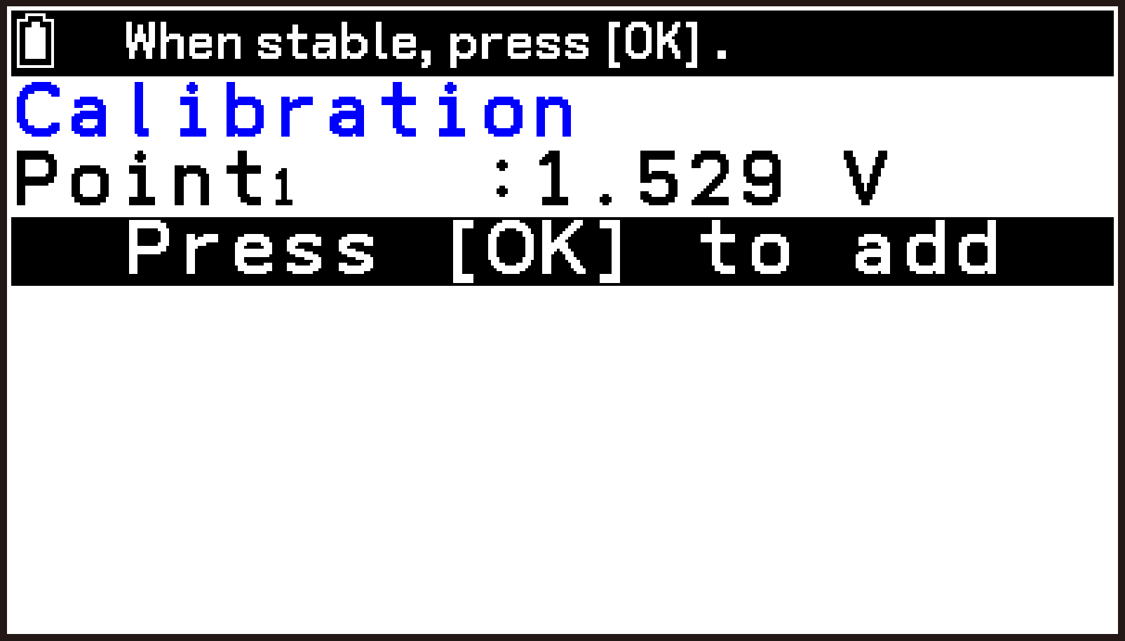
When the voltage value stabilizes, press O.
-
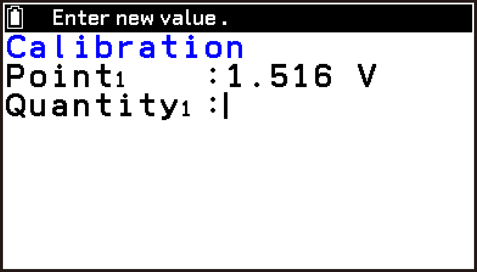
Enter a value in Quantity1, and then press O.
-
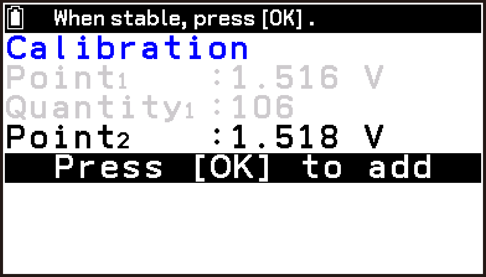
When the voltage value stabilizes, press O.
-
Press O.
-
Press u.
-
To save the calibration result, highlight
, and then press O.
Connect it to the sensor terminal (1, 2, or 3) corresponding to the channel (CH1, CH2, CH3) selected on the top screen.
This displays the Calibration screen. The Point1 row displays the current voltage value from the sensor detected by the E-CON5 app.
The voltage value at the time you press O is acquired as the Point1 value. At the same time, a row appears for entering the measurement value Quantity1 corresponding to this voltage value.
The Point1 and Quantity1 pair is registered, and the Point2 row displays the current voltage value.
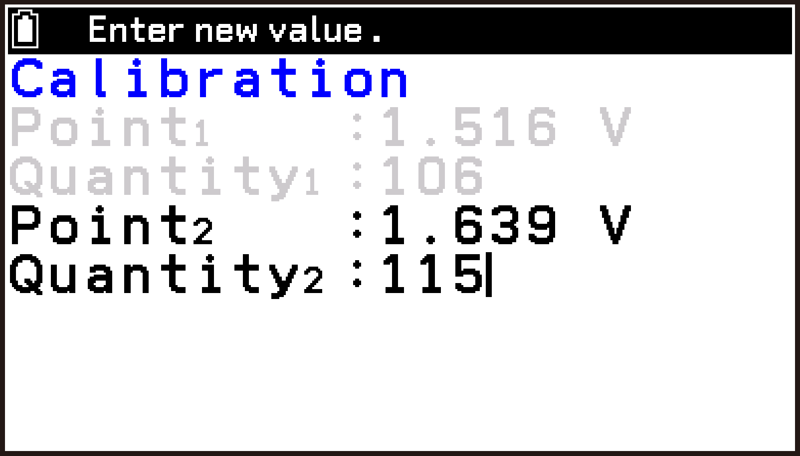
The Point2 value is acquired, and a row appears for entering the measurement value Quantity2 corresponding to the Point2 voltage value. Enter a value in Quantity2.
The Point2 and Quantity2 pair is registered, and the Properties screen reappears. This completes calibration.
Note:
If is selected for Convert, you also need to acquire a Point3 voltage value and enter a Quantity3 value.

You can confirm that the coefficient values for the function selected in Convert (in this case, ) have been automatically set by calibration.
This returns to the custom sensor file list screen.
Using a Custom Sensor
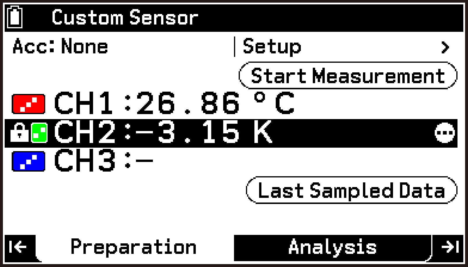
The following example explains the operation when using a custom sensor on CH2.
-
Connect the calculator and CLAB, and then start the E-CON5 app.
-
Connect the sensor you want to use as a custom sensor to CLAB sensor terminal 2.
-
Highlight CH2, and then select T > [Sensor Menu] > [Custom Sensor].
-
Highlight the custom sensor file you want to assign to CH2, and then select T > [Use Custom Sensor].
This displays the E-CON5 app top screen.
This displays the custom sensor file list screen.
This returns to the top screen. The custom sensor on CH2 is enabled for use.
To unassign a custom sensor
Highlight the channel (CH1, CH2, or CH3) to which the custom sensor is assigned, and then select T > [Sensor Menu] > [Remove Sensor].
Editing a Custom Sensor
-
Perform steps 1 through 3 under Creating a New Custom Sensor to display the custom sensor file list screen.
-
Highlight the custom sensor file you want to edit, and then select T > [Edit custom sensor].
-
On the Properties screen, edit each item as required.
-
After you are finished editing, highlight
, and then press O.
This displays the Properties screen.
For details about each item, see Custom Sensor Setting Item Details.
This returns to the custom sensor file list screen.
Deleting a Custom Sensor
-
Perform steps 1 through 3 under Creating a New Custom Sensor to display the custom sensor file list screen.
-
Highlight the file of the custom sensor you want to delete, and then select T > [Delete Custom Sensor].
-
To delete, select [OK] on the confirmation dialog.
This displays the “Delete custom sensor?” dialog.
Other Preparation Tab Operations
Changing the Measurement Range and Display Unit of a Sensor
This operation can be performed on automatically recognized sensors (including the built-in CLAB accelerometer) or on sensors selected from the library.
The following example explains how to change the measurement range of the BT05i temperature sensor included with CLAB while it is connected to CLAB sensor terminal 1.
-
Connect the calculator and CLAB, and then start the E-CON5 app.
-
Connect the temperature sensor included with CLAB to CLAB sensor terminal 1.
-
Highlight CH1, and then select T > [Sensor Menu] > [Select Range].
-
Highlight the option you want to use, and then press O.
This displays the E-CON5 app top screen.
This displays the measurement range and display unit options for the BT05i temperature sensor. The highlighted row indicates the current setting.
“EEPROM” indicates the initial default settings of the automatically recognized sensor.
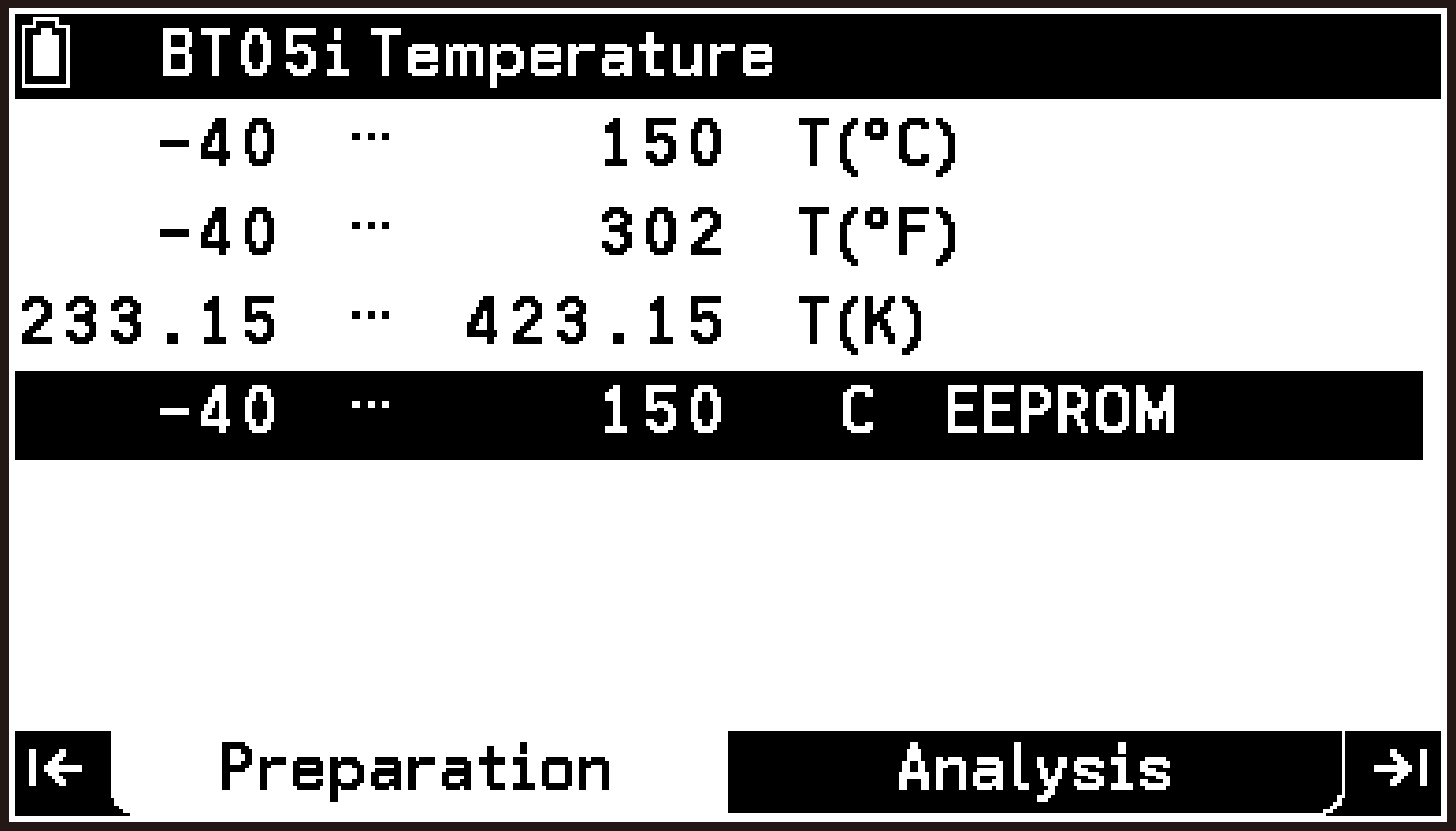
This returns to the top screen and applies the changed measurement range and display unit.
Note
For channels (CH1, CH2, or CH3) assigned a sensor selected from the library, you can change the measurement range and display unit even if no sensor is currently connected to the CLAB. To do so, highlight the corresponding channel, and then select T > [Sensor Menu] > [Select Range].
Displaying Sensor Details by Selecting a Channel
Selecting a channel (CH1, CH2, CH3, A-X, A-Y, A-Z) displays its sensor information.
-
Connect the calculator and CLAB, and then start the E-CON5 app.
-
Highlight the channel whose sensor information you want to display, and then press O. You could also select T > [Sensor Menu] > [Information].
Connect a sensor to the CLAB if required.
This displays the sensor details dialog. You can scroll the display using d or u.
Specifying the Number of Decimal Places for Displayed Values
Specifies the number of decimal places (0 through 7) for displaying sensor measurement values (Initial Default: 2). Displayed values are rounded to the number of decimal places you specify.
The following example explains how to change the number of decimal places using the BT05i temperature sensor included with CLAB, connected to CLAB sensor terminal 1.
-
Perform steps 1 and 2 under Changing the Measurement Range and Display Unit of a Sensor.
-
Highlight CH1, and then select T > [Decimal Digits].
-
On the input dialog that appears, enter an integer from 0 through 7, and then press O.
For example, if you enter “3”, measurement values are displayed with three decimal places.

Adjusting Sensor Measurements (Offset/Taring)
You can adjust sensor measurement values by applying an offset to the current reading or by resetting it to zero (taring).
To apply an offset to the current measured value
-
Connect the calculator and CLAB, and then start the E-CON5 app.
-
Connect a sensor to the CLAB.
-
On the top screen, highlight CH1, and then select T > [Edit Value] > [New Value].
-
Enter another value, and then press O.
In this example, connect the sensor to CLAB sensor terminal 1.
This displays the input dialog. The current measured value is shown in the dialog and can be edited.
This returns to the top screen. An offset is applied so that subsequent sensor measurements are adjusted according to the difference between the original value shown in the input dialog and the value you entered.
To reset the current measured value to zero (taring)
-
Perform steps 1 and 2 under To apply an offset to the current measured value.
-
On the top screen, highlight CH1, and then select T > [Edit Value] > [Reset to Zero].
This tares the sensor by resetting the current measured value to zero.
To initialize sensor calibration
After changing the current measured value to another value or resetting it to zero, you can use the following steps to reset the sensor to its initial calibration settings.
-
Perform steps 1 and 2 under To apply an offset to the current measured value.
-
On the top screen, highlight CH1, and then select T > [Edit Value] > [Reset Value].
Specifying Line Style and Color for Graph Drawing
For each channel (CH1, CH2, CH3, A-X, A-Y, A-Z), you can specify the style (graph drawing method using points or lines) and color to be used when graphing.
-
Connect the calculator and CLAB, and then start the E-CON5 app.
-
Highlight the channel for which you want to specify the line style and color for graph drawing.
-
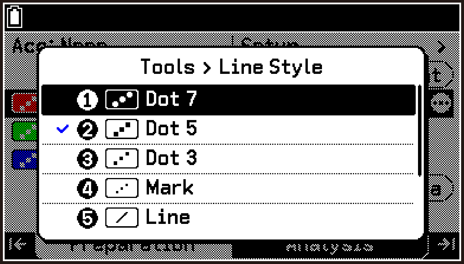
Select T > [Line Style].
-
Highlight the style you want, and then press O.
-
Select [Line Color].
-
Highlight the color you want, and then press O.
-
To return to the top screen, press b.
You can connect a sensor, if you want, but it is not required.
To specify A-X, A-Y, or A-Z, enable the accelerometer (see Using the Acceleration Sensor).
This displays the Line Style menu.
This returns to the Tools menu. Next, specify the color for graph drawing.
This displays the Line Color menu.
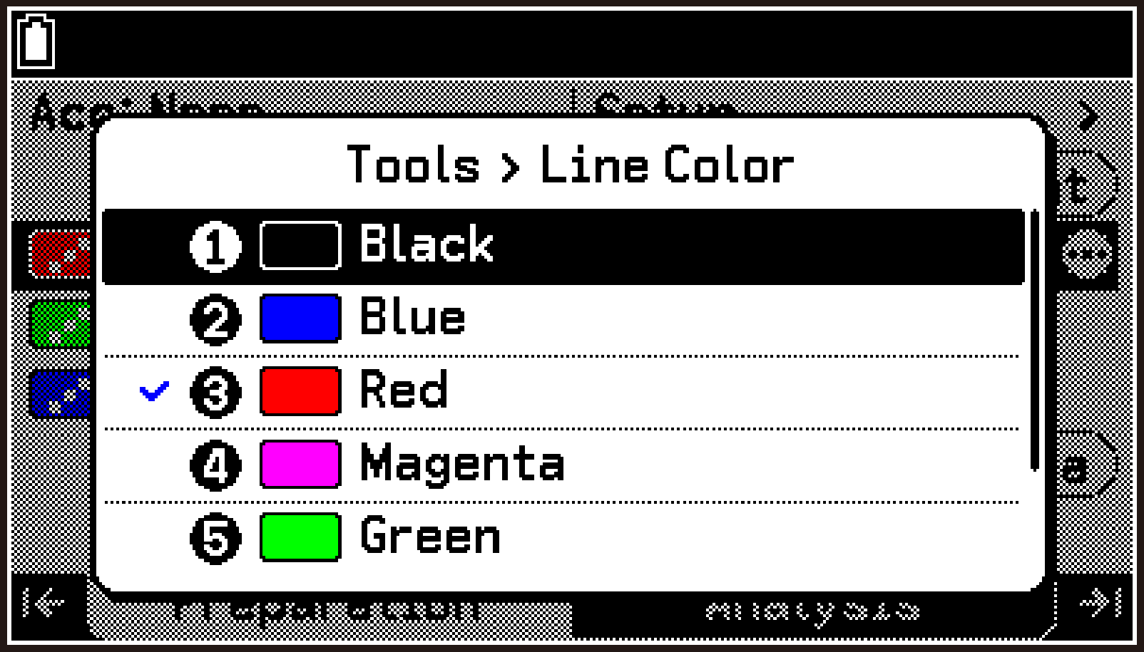
The changed settings are reflected by the icon to the left of the highlighted channel.
Graph Screen Display and Menu (Analysis Tab)
Graph Screen Display Content
On the top screen, press < or >, or highlight , and then press O to display the graph screen.
This screen displays graphs based on the data collected during measurement. The displayed graphs include “standard graphs”, which are automatically created for each channel used for measurement (CH1, CH2, CH3, A-X, A-Y, A-Z), and “custom graphs”, up to three of which can be created by you.
Standard Graph Example (CH1 Graph Screen)
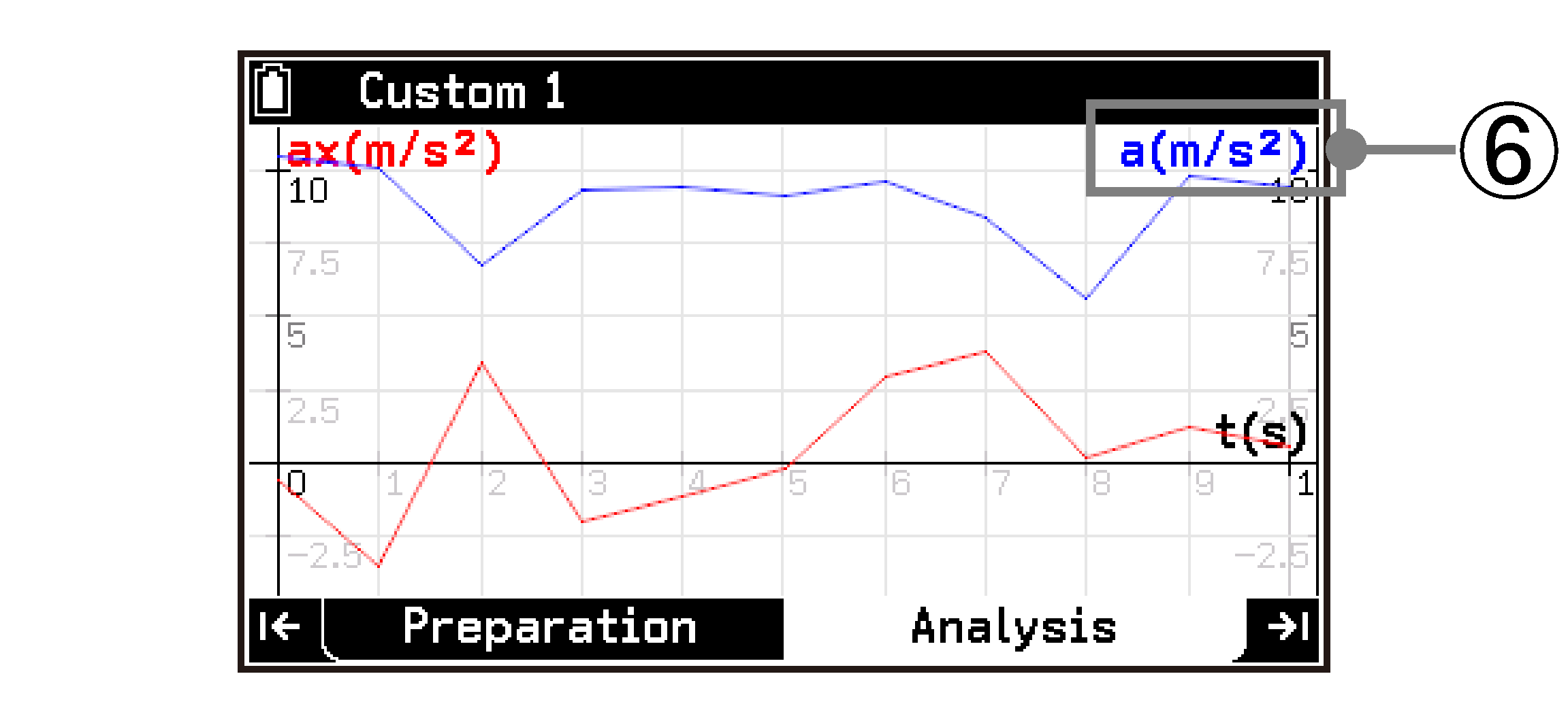
Custom Graph Example
-
Status bar showing the channel of the currently displayed graph (CH1, CH2, CH3, A-X, A-Y, A-Z), manual input data (Manual1, Manual2, Manual3), or the name of a custom graph.
-
Y-axis label of the graph
-
If a sensor is connected to the channel currently displayed on the graph screen, the current measurement value is reflected on the Y-axis.
-
The graph is drawn according to the style, color, and display range specified with T > [Graph View]. For details, see Graph Property Settings (Analysis Tab).
-
X-axis label of the graph
-
A custom graph can be configured to draw two graphs simultaneously. In this case, a second Y-axis label is displayed at the right edge of the screen. For details about custom graphs, see Creating a Custom Graph (Analysis Tab).
To switch between multiple graph screens
If multiple graph screens are available (for example, CH1, CH2, and a custom graph), use U and D to switch between them.
To scroll a graph
Use the cursor keys (d/u/l/r).
To zoom a graph display
To zoom in on the entire graph, press +. To zoom out, press -.
To zoom in vertically, press /. To zoom out vertically, press *.
To zoom in horizontally, press (. To zoom out horizontally, press ).
To return a graph to its initial display (before scrolling or zooming)
Press a.
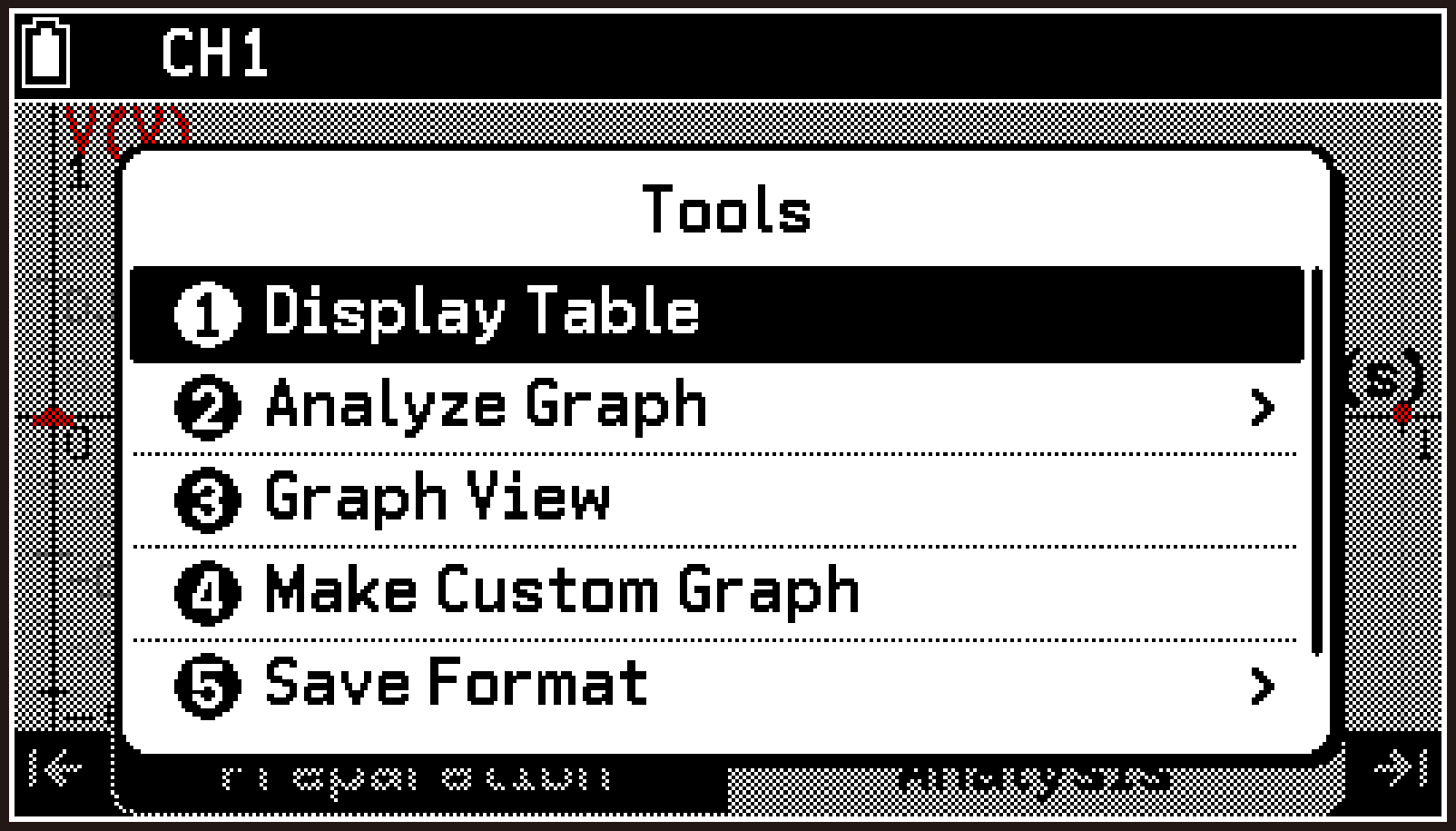
Graph Screen Tools Menu
On the graph screen, press T to display the Tools menu, which lets you analyze the currently displayed graph, change its settings, and save data.
|
For information about this Item: |
Go here: |
|
|---|---|---|
|
T > [Display Table] |
Performing a Measurement and Displaying the Results in a Graph or Table |
|
|
T > [Analyze Graph] |
||
|
T > [Graph View] |
||
|
T > [Make Custom Graph] |
||
|
T > [Delete Custom Graph] |
||
|
T > [Save Format] > |
[List] |
|
|
[CSV] |
||
|
T > [Start Measurement] |
To start a new measurement while the graph or table screen is displayed |
|
Table Screen Display and Menu (Analysis Tab)
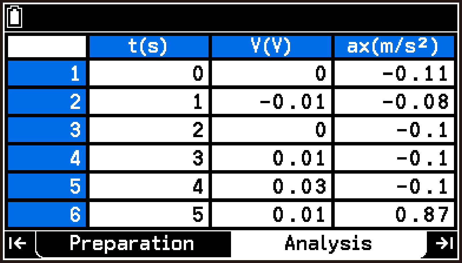
Table Screen Display Content
On the graph screen, select T > [Display Table] to display the table screen. This screen shows the data collected during measurement (and data entered manually) in table format.
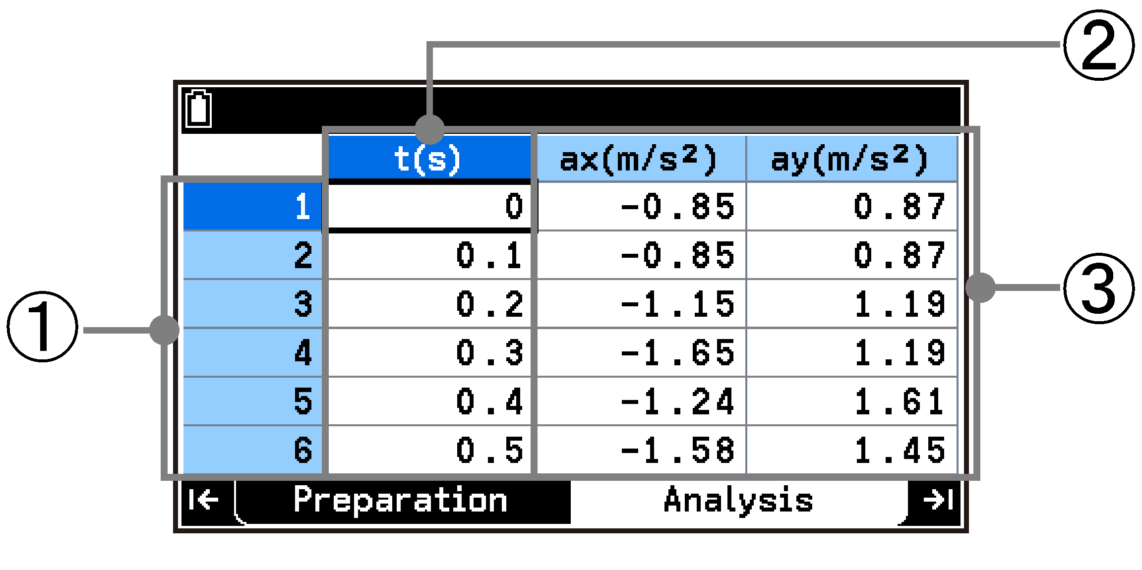
-
Row numbers: Indicate the sample numbers in the data collection sequence. The last row number corresponds to the total number of samples.
-
First data column: This is the X-axis data of the graph. If the measurement type is “Time-based”, the data is time. If the measurement type is “Manual” or “Interval”, the data is an index (data sequential number).
-
Second and subsequent data columns: This is the Y-axis data of the graph. Column headers show the quantity symbols and units of the measured data. For example:
The standard column header name is “t(s)” when the measurement type is “Time-based”, and “n” when the measurement type is “Manual” or “Interval”.
T(°C) ... Quantity symbol: T (temperature), Unit: °C
ax(m/s2) ... Quantity symbol: ax (acceleration in the -axis direction), Unit: m/s2
Δt(s) ... Quantity symbol: Δt (time interval), Unit: s
To return from the table screen to the graph screen, press b. Note that pressing < or > on the table screen does not display the Preparation tab (top screen), but instead returns to the graph screen.
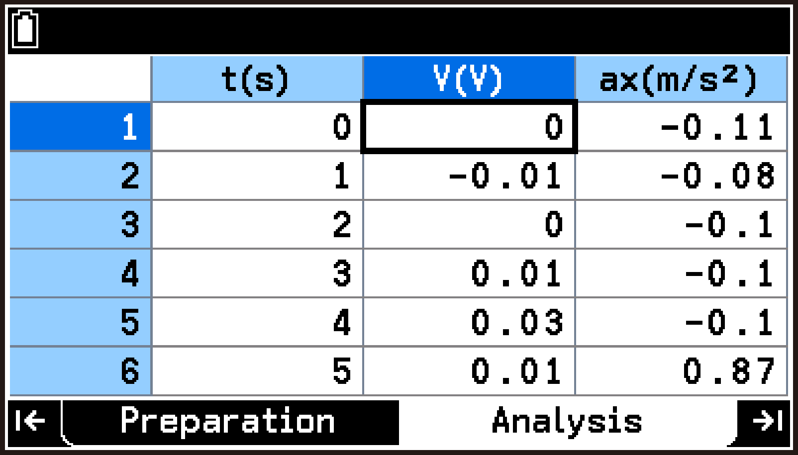
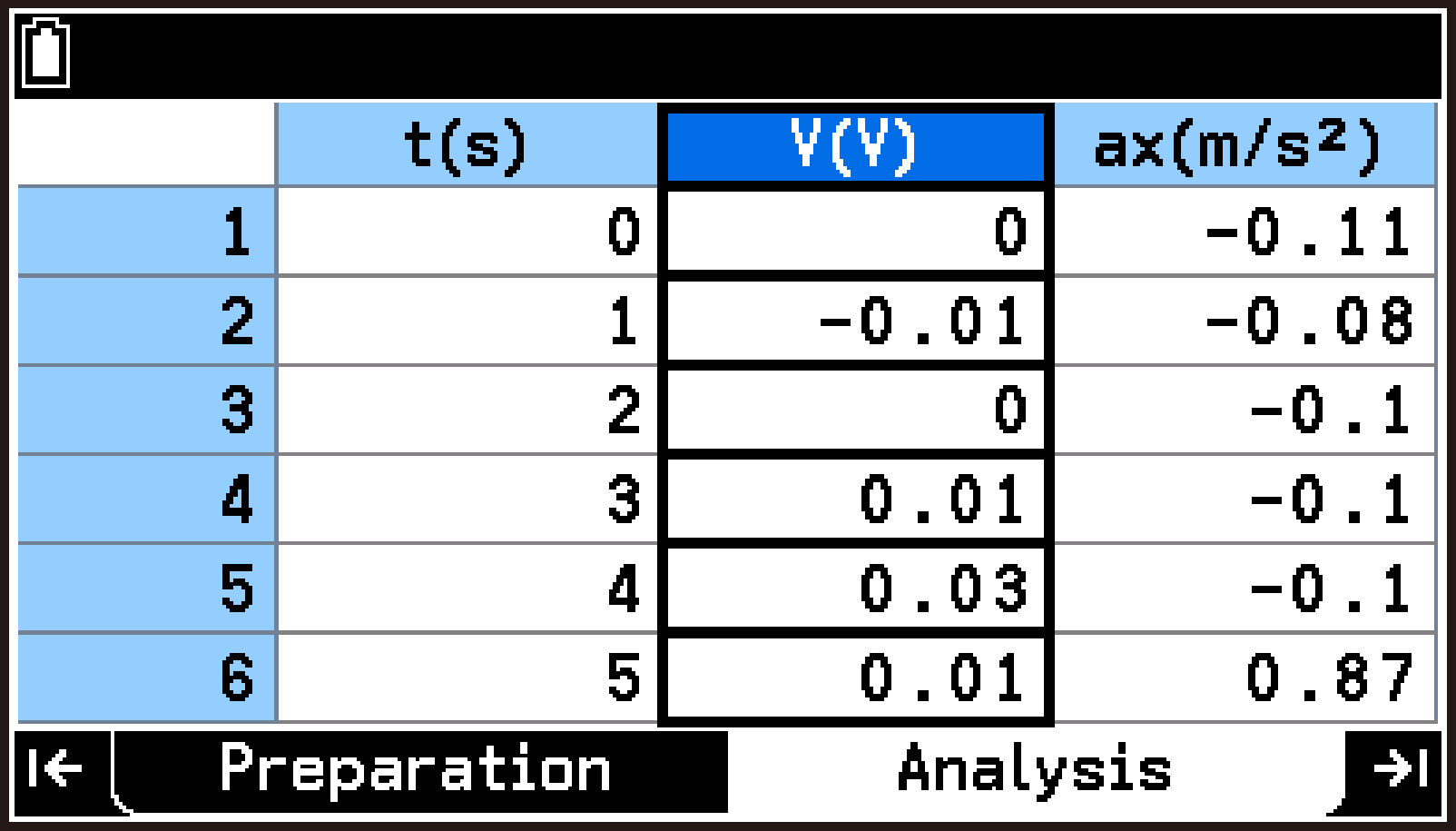
Selecting a Specific Column or All Cells on the Table Screen
To select a specific column on the table screen
Move the cursor to the top cell of the column you want to select, and then press u.
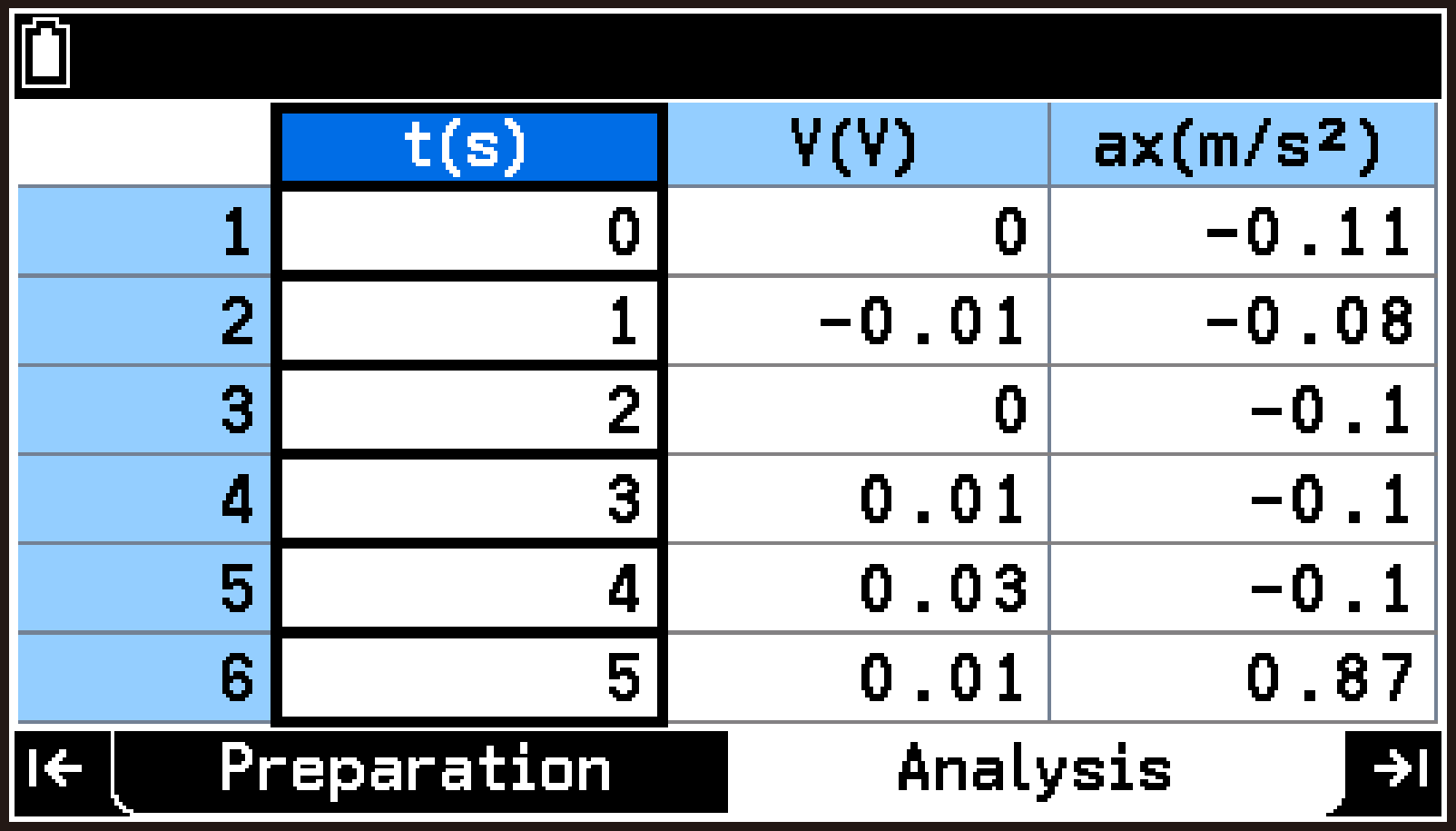
To select all cells on the table screen
Select the entire leftmost column, and then press l.
Note
When saving measurement data, select cells as required using the above operations.
Table Screen Tools Menu
On the table screen, press T to display the following Tools menu.
|
For information about this Item: |
Go here: |
|
|---|---|---|
|
T > [Save Format] > |
[List] |
|
|
[CSV] |
||
|
T > [Start Measurement] |
To start a new measurement while the graph or table screen is displayed |
|
|
T > [Advanced Function] > [Ball Bounce] |
||
Graph Analysis (Analysis Tab)
This section explains how to use the graph analysis tools included on the Analyze Graph menu.
|
For information about this Item: |
Go here: |
|---|---|
|
T > [Analyze Graph] > [Trace] |
|
|
T > [Analyze Graph] > [Average] |
|
|
T > [Analyze Graph] > [Change in values] |
Displaying the Change in Data Values for a Specified Interval |
|
T > [Analyze Graph] > [Slope] |
|
|
T > [Analyze Graph] > [Signed area sum] |
|
|
T > [Analyze Graph] > [Fit] |
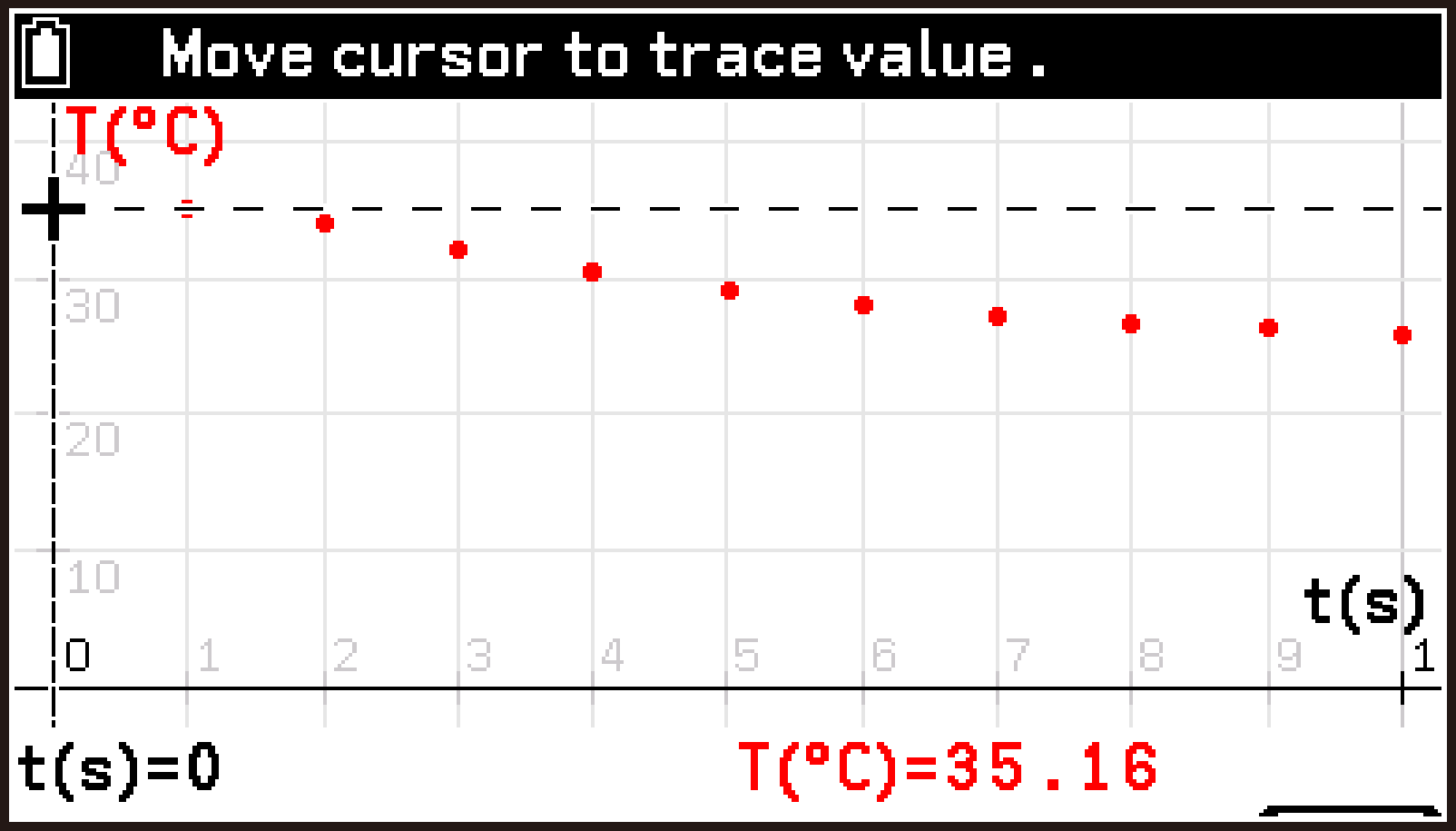
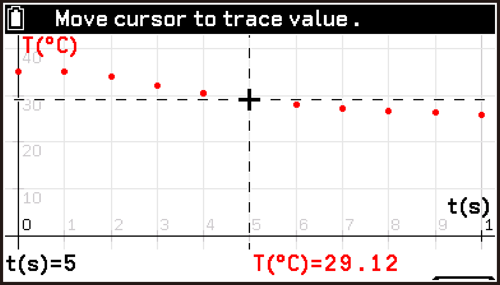
Using Trace
Trace displays the coordinate values of data points (points representing each sample value) on a graph.
-
On the graph screen, select T > [Analyze Graph] > [Trace].
-
To display the coordinate values of another data point, move the pointer using l or r.
-
To exit Trace, press b.
A pointer (+) appears at the first data point of the graph, and the coordinate values of that point are displayed at the bottom of the screen.
Displaying the Mean Value of Data in a Specified Interval
Use this procedure to specify two data points on the graph and display the mean value of the data in that interval.
-
On the graph screen, select T > [Analyze Graph] > [Average].
-
Use l and r to move the pointer to the location you want to specify, and then press O.
-
Use l and r to move the pointer to the location you want to specify as the end point, and then press O.
-
To complete the operation, press b.
This causes a pointer to appear at the start point of the current interval.*
The X-axis coordinate of the current pointer position is displayed in the lower left corner of the screen.
The mean value of the data in the currently specified interval is displayed on the lower right corner of the screen.
This causes the pointer to move to the end point of the interval.
This displays the mean value of the specified interval in the lower right corner of the screen.
Each press of O moves the pointer between the start point and end point. You can repeat steps 2 and 3 to display the mean value of another interval.
The pointer position from the last time a graph analysis tool was used is remembered. For this reason, the pointer may initially appear at the end point.
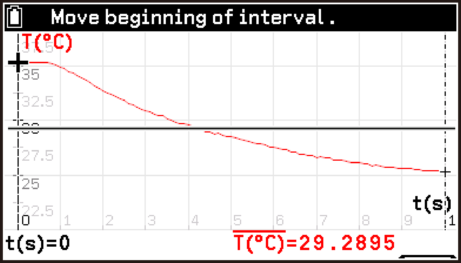
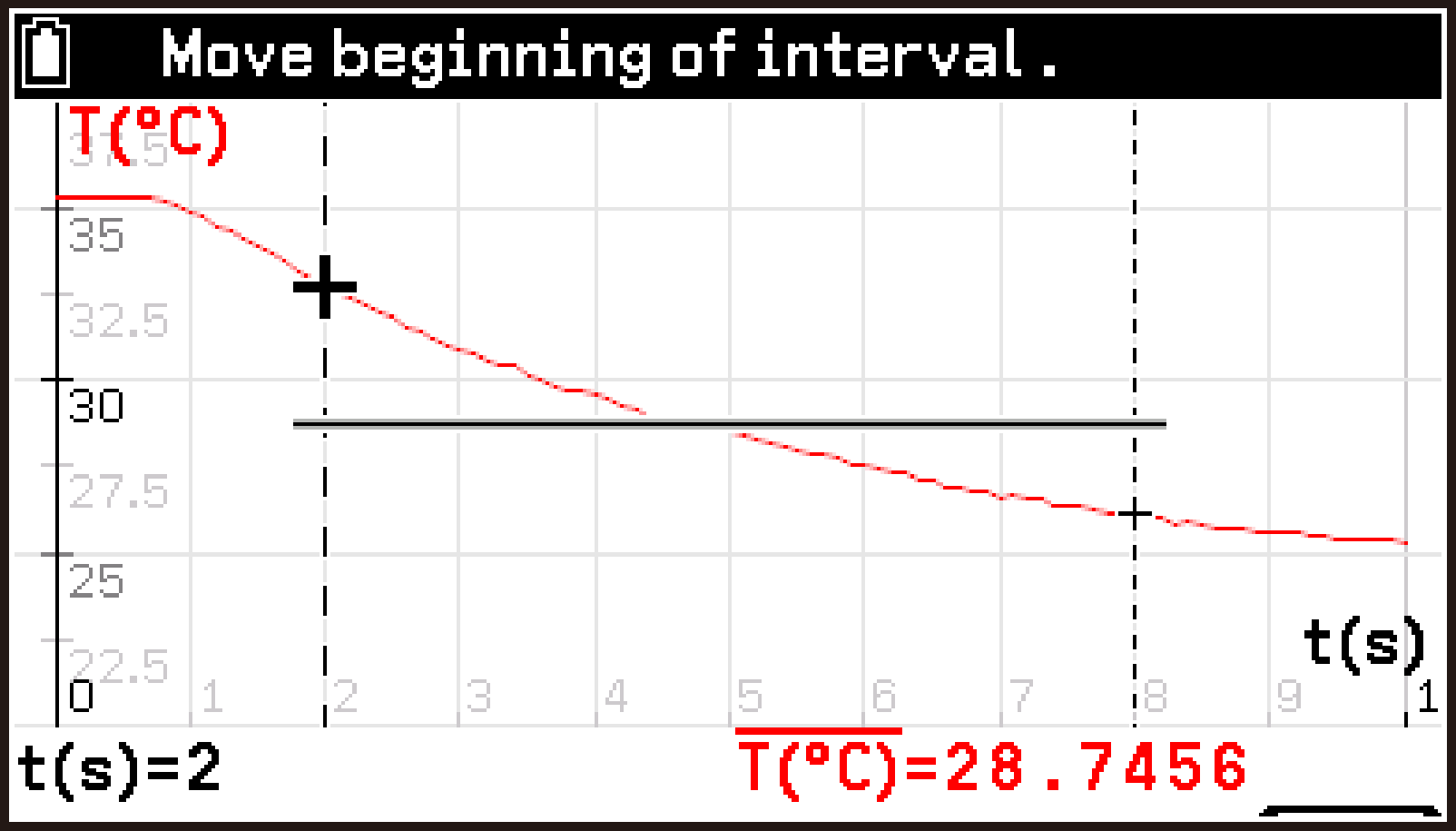
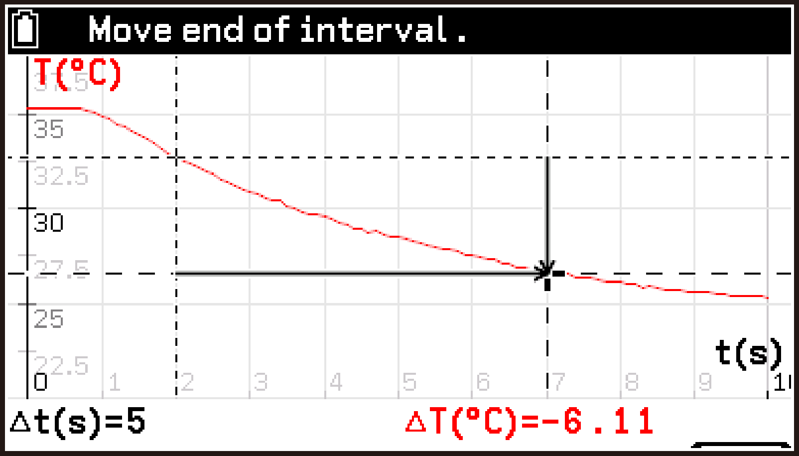
Displaying the Change in Data Values for a Specified Interval
Use this procedure to specify two data points on the graph and display the change in data values for the interval on both the X-axis and Y-axis.
-
On the graph screen, select T > [Analyze Graph] > [Change in values].
-
Use l and r to move the pointer to the location you want to specify, and then press O.
-
Use l and r to move the pointer to the location you want to specify as the end point, and then press O.
-
To complete the operation, press b.
This displays a pointer at the start point of the current interval.
This causes the pointer to move to the end point of the interval.
This causes the change in data values for the specified interval to appear at the bottom of the screen.
Lower left: Change in X-axis data values
Lower right: Change in Y-axis data values
Each press of O moves the pointer between the start point and end point. You can repeat steps 2 and 3 to display the change in data values for another interval.
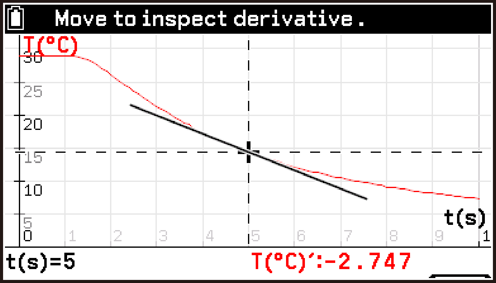
Drawing a Tangent on a Graph and Displaying the Slope Value
Use this procedure to draw a tangent on a specified data point of the graph and display the slope (derivative) value of the tangent.
-
On the graph screen, select T > [Analyze Graph] > [Slope].
-
Use l and r to move the pointer.
-
To complete the operation, press b.
This displays a pointer for specifying a data point, draws a tangent at that point, and displays the slope value of the tangent in the lower right corner of the screen.
This lets you observe how the tangent and slope value change according to the pointer position.
Note
When calculating the slope value with the above operation, the E-CON5 app applies a smoothing process to the measurement data (averaging multiple data points around the specified point). This is especially important when the measurement data contains a large amount of noise. However, depending on the state of the measurement data and the point you specify, unexpected calculation results may be displayed.
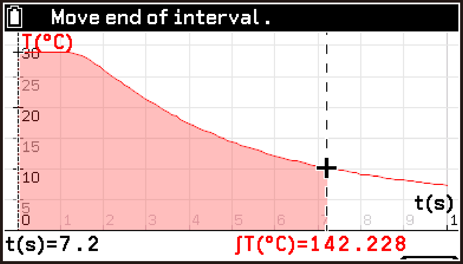
Displaying the Area of a Specified Interval
Use this procedure to specify two data points on a graph and display the area (integral value) enclosed by the graph and the X-axis for the interval.
-
On the graph screen, select T > [Analyze Graph] > [Signed area sum].
-
Use l and r to move the pointer to the location you want to specify, and then press O.
-
Use l and r to move the pointer to the location you want to specify as the end point, and then press O.
-
To complete the operation, press b.
This displays a pointer at the start point of the current interval.
The X-axis coordinate of the current pointer position is displayed in the lower left corner of the screen.
The area of the current interval appears in the lower right corner of the screen.
This causes the pointer to move to the end point of the interval.
This displays the area value of the specified interval in the lower right corner of the screen.
Each press of O moves the pointer between the start point and end point. You can repeat steps 2 and 3 to display the area of another interval.
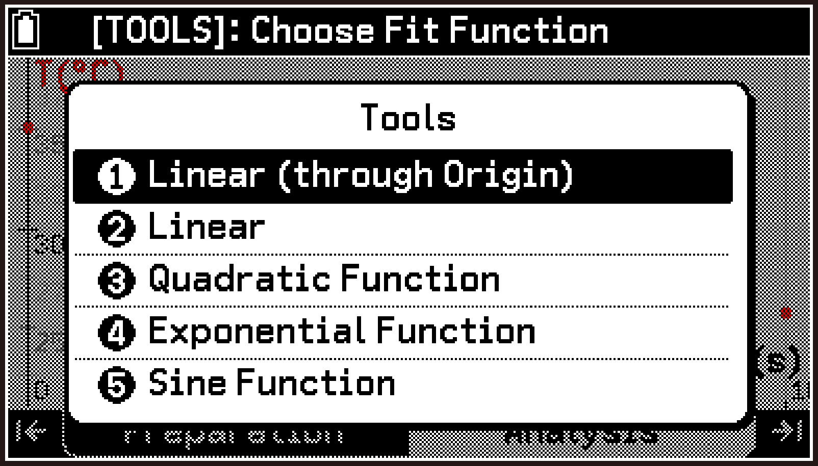
Fitting Data on a Graph to a Standard Function
Use this procedure to specify an interval on a displayed graph and approximate the data in that interval using one of the following functions.
Linear (through Origin) ... Linear function passing through the origin ()
Linear ... Linear function ()
Quadratic Function ... Quadratic function ()
Exponential Function ... Exponential function ()
Sine Function ... Sine function ()
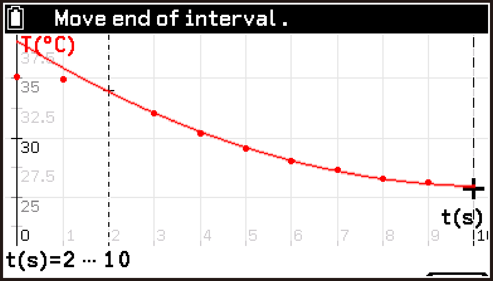
The following example describes fitting a quadratic function.
-
On the graph screen, select T > [Analyze Graph] > [Fit].
-
Press T.
-
Highlight the function you want to use (here, Quadratic Function), and then press O.
-
Use l and r to move the pointer to the location you want to specify as the start point.
-
When the pointer is at the location you want, press O.
-
Use l and r to move the pointer to the location you want to specify as the end point, and then press O.
-
After specifying the start point and end point, press b.
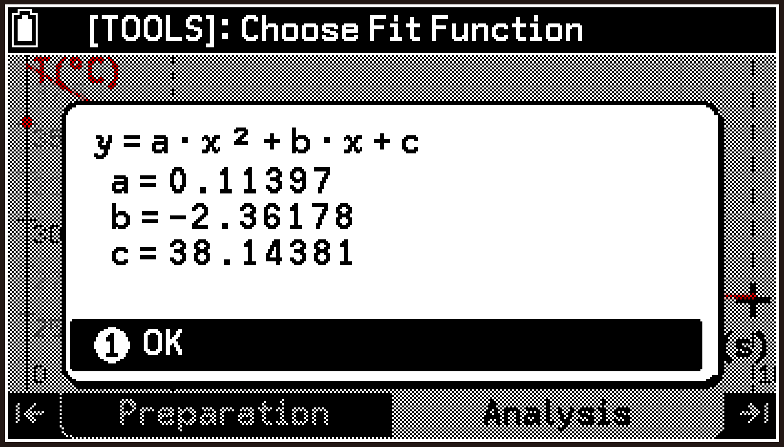
-
Select T > [Information].
-
To close the dialog, press O.
-
To complete the operation, press b.
This causes the message “[TOOLS]: Choose Fit Function” to appear in the status bar.
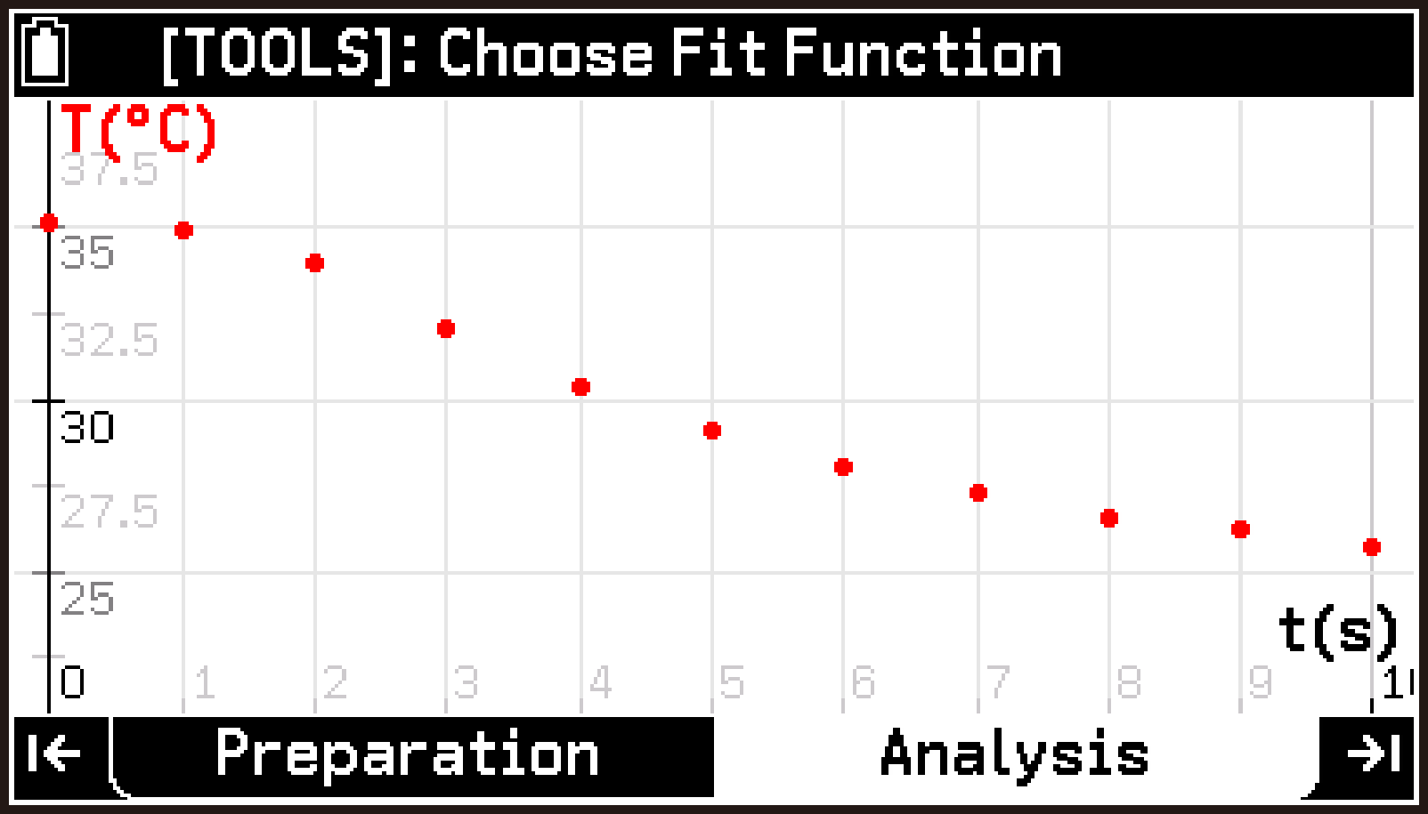
This displays a menu of available functions.
This displays a pointer at the start point of the current interval.
The currently specified interval is shown in the lower left corner of the screen. A quadratic curve approximating the data for the currently specified interval is drawn on top of the graph displayed in step 1.
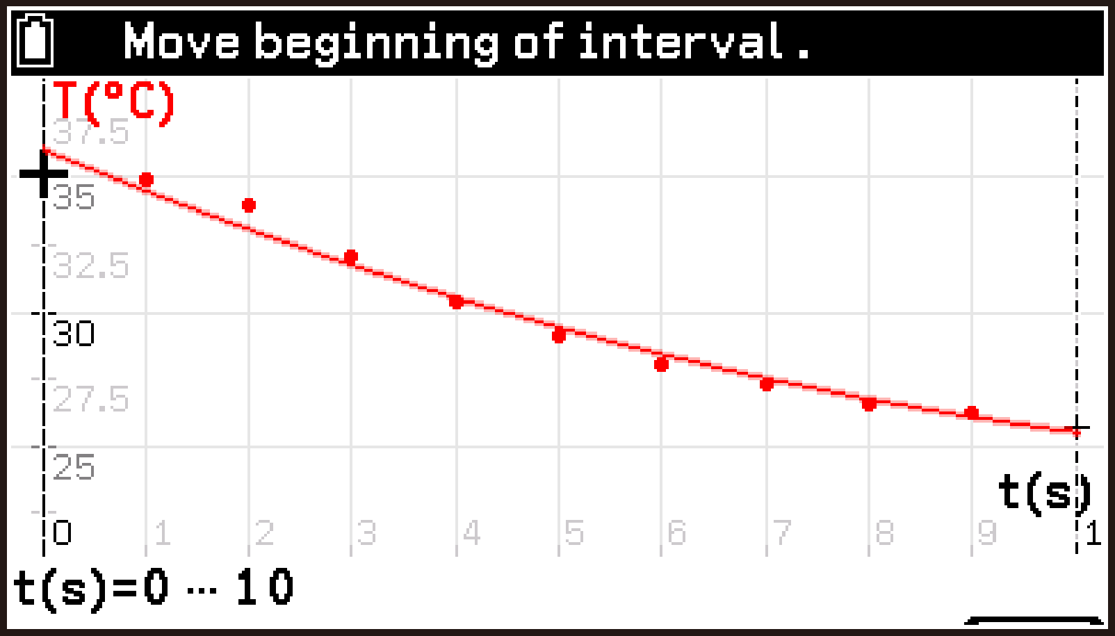
Moving the pointer changes the data range used for the calculation, which causes the shape of the fitted graph to change accordingly.
This causes the pointer to move to the end point of the interval.
Each press of O moves the pointer between the start point and end point. You can repeat steps 4 through 6 as needed to adjust the interval.
This causes the message “[TOOLS]: Choose Fit Function” to appear in the status bar.
This displays a dialog with the coefficient values of the fitted curve.
Note
The Fit feature of the E-CON5 app provides a simple way to approximate measurement data with a function. For more advanced analysis, the Statistics app or the Spreadsheet app lets you apply a wider range of regression models and view more detailed calculation results.
Perform the following steps to analyze measurement data using these apps.
Statistics app:
-
Save the measurement data to a list variable.
-
Start the Statistics app.
-
Using the list variable saved in step 1 above, do one of the following:
See Saving Measurement Data to a List Variable.
Display regression model information. For details, see Displaying Summary Statistics or Regression Model Information.
Draw a regression graph. For details, see Drawing a 2-Variable Statistics Graph (Scatter Plot or Regression Graph).
Spreadsheet app:
-
Save the measurement data to a CSV file.
-
Start the Spreadsheet app.
-
Import the CSV file saved in step 1 into the Spreadsheet app.
-
Do one of the following:
See Saving Measurement Data to a CSV File.
See To import a CSV file into a spreadsheet (Spreadsheet app).
Display regression model information. For details, see Displaying Summary Statistics or Regression Model Information.
Draw a regression graph. For details, see Drawing a 2-Variable Statistics Graph (scatter plot or regression graph).
Graph Property Settings (Analysis Tab)
The Graph View screen lets you configure the properties (such as display range and drawing color) of all graphs that can be displayed on the graph screen.*
This includes both standard graphs and custom graphs. For details about standard graphs and custom graphs, see Graph Screen Display Content.
Configuring the Properties of the Currently Displayed Graph
-
Display the graph screen.
-
Use U or D to display the graph whose properties you want to configure.
-
Select T > [Graph View].
-
On the Graph View screen, configure the settings of each item from Name through Grid.
-
To complete the operation, press b.
This displays the Graph View screen.
The first row of the setting item (highlighted in the example screen to the right) shows the fixed name* of the graph you displayed in step 2.
Standard Graph:
CH1, CH2, CH3, A-X, A-Y, A-Z, Manual1, Manual2, Manual3
Custom Graph:
Custom 1, Custom 2, Custom 3

For details about each item, see Graph Property Items.
When any row is highlighted, pressing a resets all axis Minimum and Maximum values to their initial defaults.
A graph’s fixed name is its initial default name. You can use Name on the Graph View screen to change the display name (shown in the status bar of the graph screen), but the fixed name shown in the first row of the Graph View screen does not change.
Note
You can continue configuring the properties of other graphs without pressing b in step 5. To do so, perform the following operation.
-
Highlight row 1 of the setting items, and then press O.
-
On the menu that appears, select the graph whose properties you want to configure.
-
Configure the settings of each item from Name through Grid.
Repeat steps (1) through (3) as required. To complete the operation, press b.
Graph Property Items
In the explanations, options and values marked with “◆” are initial defaults.
Name
Highlight this item and then press O. On the dialog that appears, enter up to eight characters as the name of the graph. The name you input here is displayed in the graph screen status bar. (The channel name displayed on the top screen is not affected.)
X-axis
Standard Graph:
If the measurement type is Manual or Interval, this item is fixed as Index(n).
When the measurement type is Time-based, you can select this item and then press O to display a sub-menu that includes the following menu items.
X-axis > [Change Unit]
Specifies the measurement time unit displayed on the graph.
Time(ms) (milliseconds), Time(s)◆ (seconds), Time(min) (minutes), Time(hour) (hours)
Custom Graph:
Highlighting this item and pressing O displays the following sub-menu.
X-axis > [Assign Variables]
Specifies the data to be assigned to the X-axis of the custom graph. The initial default is Time(s) if the measurement type is Time-based, or Index(n) if the measurement type is Manual or Interval. For options other than the defaults, see List of Data Assignable to the X-axis and Y-axis in a Custom Graph.
X-axis > [Change Unit] (Time-based measurement type only)
You can select one of the following as the measurement time unit displayed on the graph.
Time(ms) (milliseconds), Time(s)◆ (seconds), Time(min) (minutes), Time(hour) (hours)
Minimum, Maximum
Enter the minimum and maximum values to be displayed on the X-axis. You can enter values in the range of -360,000 to 360,000. The initial defaults are automatically adjusted values according to the measurement data.
Order
This item is displayed only when the measurement type is Manual or Interval.
Highlight this item and then press O. On the menu that appears select one of the following options.
By time◆: Displays the data on the X-axis in index value order.
By value: Displays the data on the X-axis in ascending order of Y-axis measurement values.
Y-axis
For standard graphs, this item has no direct operation. Instead, you can configure Minimum, Maximum, Style, and Color under this item as needed.
For a custom graph, highlight this item and then press O. Use the menu that appears to specify the data to be assigned to the Y-axis of the custom graph. For information about selectable options, see List of Data Assignable to the X-axis and Y-axis in a Custom Graph.
Minimum, Maximum
Enter the minimum and maximum values to be displayed on Y-axis. You can enter values in the range of -100,000 to 100,000. The initial defaults are automatically adjusted values according to the measurement data.
Style
Highlight this item and then press O. Use the menu that appears to specify the drawing style (points and lines used for drawing).
Color
Highlight this item and then press O. Use the menu that appears to select the graph drawing color.
Y2-axis
The settings of this item can be configured only for custom graphs. When you want to display two graphs at the same time, highlight this item and then press O. Use the menu that appears to assign the data for the second graph. The initial default is None (do not display a second graph). For options other than the defaults, see List of Data Assignable to the X-axis and Y-axis in a Custom Graph. If you specify any option other than None, the following items appear under Y2-axis: Minimum, Maximum, Style, and Color. These settings are the same as those under Y-axis.
Grid
Highlight this item and then press O. Use the menu that appears to specify show or hide for the graph screen grid.
Off: Hide graph screen grid.
On◆: Show graph screen grid.
List of Data Assignable to the X-axis and Y-axis in a Custom Graph
On the Graph View screen of a custom graph, select X-axis > [Assign Variables], or highlight Y-axis or Y2-axis and then press O. This displays a menu like the following (Example: X-axis).
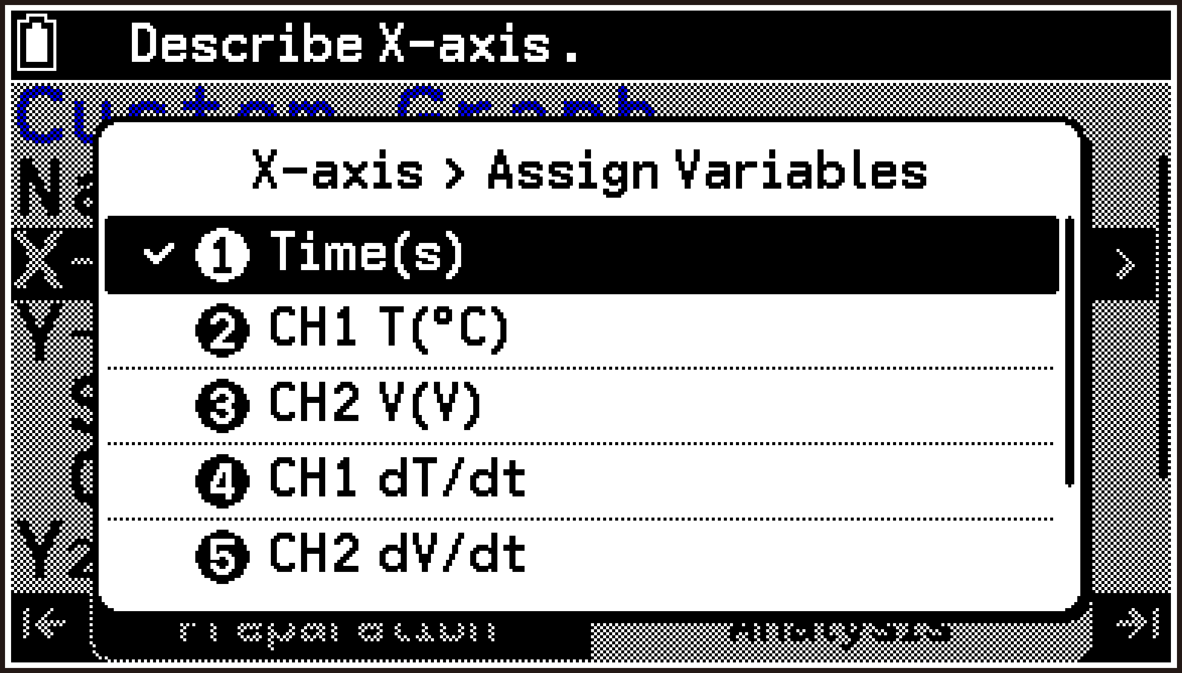
Use this menu to assign data to each axis. The table below lists all available options.
In this table, “” represents the quantity symbol of the measurement data, while “” represents the unit of the measurement data.
Only the options relevant to the current measurement data are actually displayed. For example, if the current measurement data consists only of temperature measured with CH1 (quantity symbol: T, unit: °C), the menu shows [CH1 T(°C)], [CH1 dT/dt], and [CH1 d2T/ dt2].
|
Option |
Description |
|---|---|
|
CH1 () CH2 () CH3 () |
CH1, CH2, CH3 measurement data. The quantity symbol and unit vary depending on the connected sensor. |
|
A-X ax(m/s2) A-Y ay(m/s2) A-Z az(m/s2) |
CLAB built-in accelerometer measurement data. |
|
Man1 () Man2 () Man3 () |
Manually entered data when the measurement type is Manual. Quantity symbols and units depend on user settings. For details, see Manual Type Setting Items. |
|
CH1 d/dt CH2 d/dt CH3 d/dt |
First derivative of CH1, CH2, CH3 measurement data. |
|
v(m/s) |
Velocity calculated using measurements from the motion sensor (BT55i). This option is displayed only when at least two BT55i sensors are connected. |
|
CH1 d2/ dt2 CH2 d2/ dt2 CH3 d2/ dt2 |
Second derivative of CH1, CH2, CH3 measurement data. |
|
a(m/s2) |
Acceleration calculated using measurements from the motion sensor (BT55i). This option is displayed only when at least two BT55i sensors are connected. |
|
Sum of A-(X,Y,Z) |
Acceleration calculated using the CLAB built-in accelerometer. This option is displayed only when at least two axes (A-X, A-Y, A-Z) are enabled. |
Creating a Custom Graph (Analysis Tab)
In addition to the standard graphs automatically created each time a measurement is performed, you can create up to three custom graphs based on your own settings.
To create a custom graph
-
On the graph screen, select T > [Make Custom Graph].
-
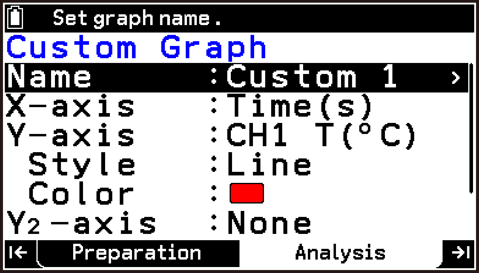
Specify the settings of each item from Name through Grid.
-
To create the custom graph with the currently configured settings, highlight
, and then press O.
This displays the Custom Graph screen.
For details about each item, see Custom Graph Setting Item Details.
This displays the custom graph on the graph screen. The status bar shows the name you input for Name.
Note
If three custom graphs already exist, [Make Custom Graph] does not appear in the menu even if you press T. To create a new custom graph in this case, delete one of the current custom graphs in memory using the procedure under Deleting a Custom Graph.
Custom Graph Setting Item Details
Name
Highlight this item and then press O. On the dialog that appears, enter up to eight characters as the name of the graph. The name you input here is displayed in the graph screen status bar.
X-axis > [Assign Variables]
Specifies the data to be assigned to the X-axis of the custom graph. The initial default is Time(s) if the measurement type is Time-based, or Index(n) if the measurement type is Manual or Interval. For options other than the defaults, see List of Data Assignable to the X-axis and Y-axis in a Custom Graph.
Y-axis
Specifies the data to be assigned to the Y-axis of the custom graph. For information about selectable options, see List of Data Assignable to the X-axis and Y-axis in a Custom Graph.
Style
Highlight this item and then press O. Use the menu that appears to specify the drawing style (points and lines used for drawing). The initial default is Line.
Color
Highlight this item and then press O. Use the menu that appears to select the graph drawing color. The initial defaults are: Custom 1: Black, Custom 2: Blue, Custom 3: Red.
Y2-axis
When you want to display two graphs at the same time, highlight this item and then press O. Use the menu that appears to assign the data for the second graph. The initial default is None (do not display a second graph). For options other than the defaults, see List of Data Assignable to the X-axis and Y-axis in a Custom Graph. If you specify any option other than None, the following items appear under Y2-axis: Style and Color. These settings are the same as those for Y-axis.
Grid
Highlight this item and then press O. Use the menu that appears to specify show or hide for the graph screen grid.
Off: Hide graph screen grid.
On: Show graph screen grid (initial default).
Deleting a Custom Graph
-
Display the graph screen.
-
Use U and D to display the custom graph you want to delete.
-
Select T > [Delete Custom Graph].
-
To delete, select [OK] on the confirmation dialog.
This displays the “Delete Custom Graph?” dialog.
Saving Measurement Data (Analysis Tab)
You can use the procedures in this section to save the measurement data currently displayed on the graph screen or table screen to a list variable or a CSV file.
When saving from the graph screen, the data of the graph currently displayed is saved. When saving from the table screen, you can either save all displayed columns together or select specific columns to save.
Custom Graph Data Save Precautions
The X-axis and Y-axis of a custom graph can be assigned data calculated from measurement data as the following.
CH1 d/dt, CH2 d/dt, CH3 d/dt, CH1 d2/ dt2, CH2 d2/ dt2, CH3 d2/ dt2, v(m/s), a(m/s2), Sum of A-(X,Y,Z)
To save any of these data items to a list variable or CSV file, be sure to save it from the graph screen. These data items are not displayed on the table screen.
For details about the meaning of each data item above, see List of Data Assignable to the X-axis and Y-axis in a Custom Graph.
Saving Measurement Data to a List Variable
-
Display the graph or table screen.
-
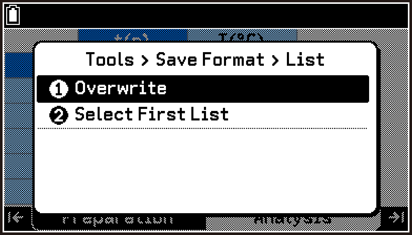
Select T > [Save Format] > [List].
-
Here, select T > [Overwrite].
-
Select h > Statistics to start the Statistics app.
When saving from the graph screen, only the data of the currently displayed graph is saved.
When saving from the table screen, you can save all displayed columns or specify particular columns.
If you select all cells or a single cell: all columns of data are saved.
If you select the entire leftmost column: only the data in the leftmost column (X-axis data) is saved.
If you select any entire column other than the leftmost: the leftmost column (X-axis data) and the selected column (Y-axis data) are both saved.
For information about selecting cells, see Selecting a Specific Column or All Cells on the Table Screen.
This displays a menu for selecting how the data will be saved.
Overwrite … Overwriting starts from List 1. For example, if the table has two columns, List 1 and List 2 are overwritten with the measurement data. (Existing list variables from List 3 onward are retained.)
Select First List … Specify the list number from which overwriting starts. For example, if you specify 3 and the table has two columns, List 3 and List 4 are overwritten with the measurement data. (The contents of other existing list variables are retained.)
This saves the measurement data to list variables and displays a confirmation dialog.
The example dialog to the right shows that t(s) (time data in seconds) is saved in List 1 and T(°C) (temperature data in Celsius) is saved in List 2.
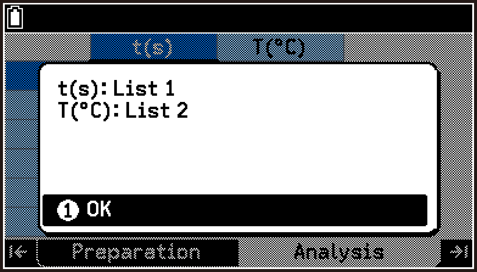
You can use the List Editor screen that appears to check the saved list variables.
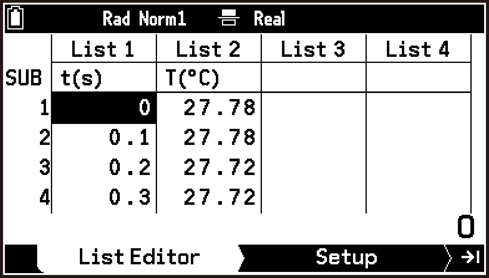
Note
The maximum number of elements in a list variable is 999. If you attempt to save measurement data with more than 999 samples, the following warning message appears. Press O to save the data up to the 999th sample.
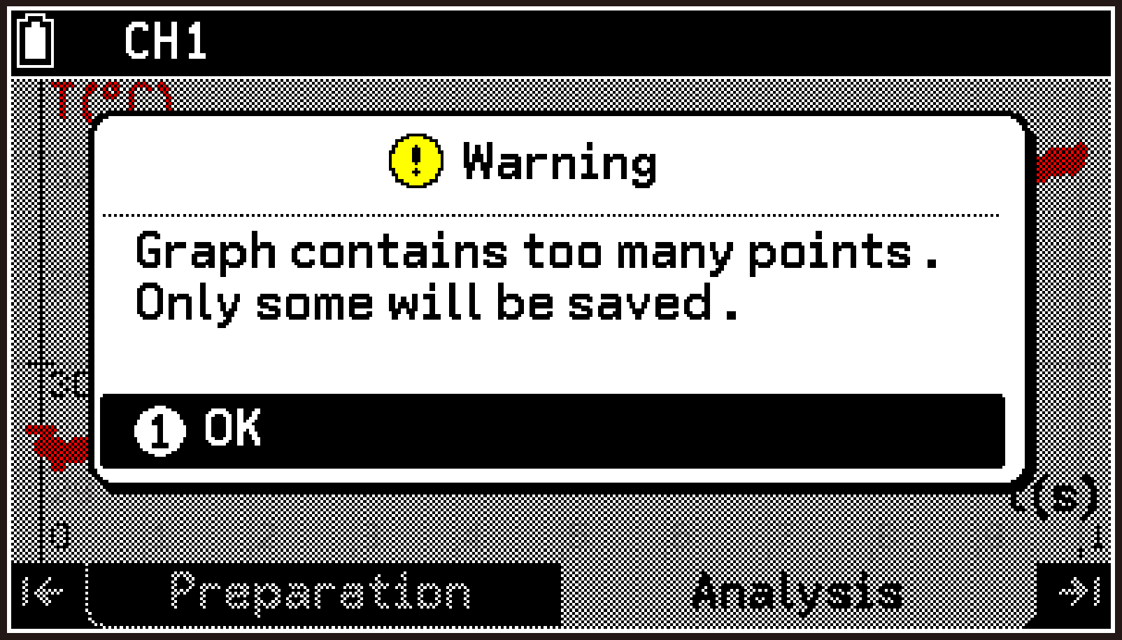
Saving from the graph screen
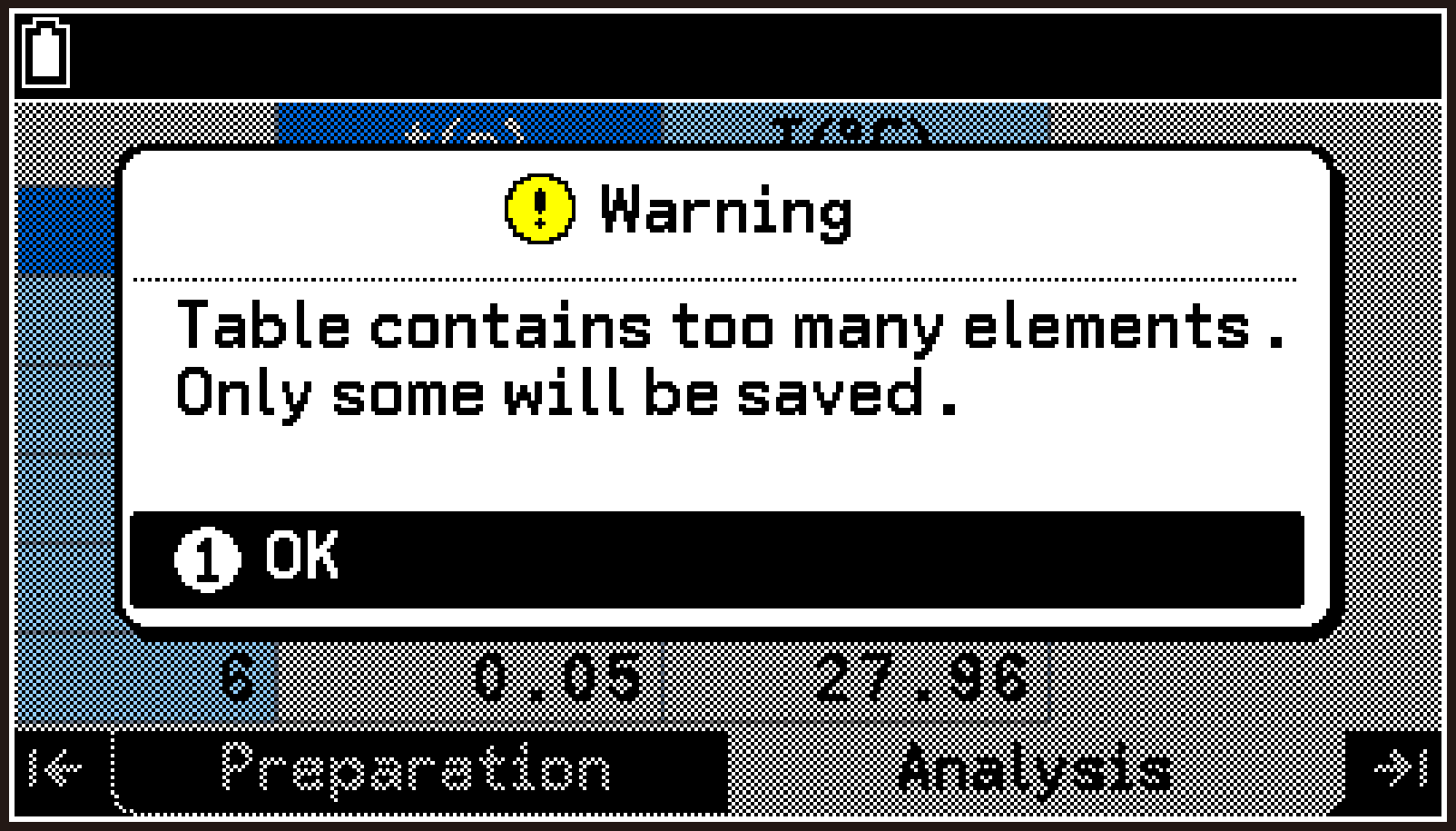
Saving from the table screen
Saving Measurement Data to a CSV File
-
Display the graph or table screen.
-
Select T > [Save Format] > [CSV].
-
Enter a filename of up to eight characters, and then press O.
For operations from each screen, see step 1 under Saving Measurement Data to a List Variable.
This displays the filename input dialog.
For information about the CSV file save destination, see E-CON5 App Data Storage.
Note
The delimiter and decimal point used when saving a CSV file with the above procedure are in accordance with the settings of the System app. For details about these settings, see Specifying the CSV File Import and Export Format (CSV Format).
The first row of a saved CSV file contains strings representing quantity symbols and units (such as t(s) or T(°C)). However, some symbols such as “°C” use calculator-specific fonts and may not display correctly when the CSV file is opened on a computer.
Using Ball Bounce (Analysis Tab)
Prepare an experiment setup like the one shown to the right, in which a ball is dropped, lands on the floor, and bounces back. You can analyze measurement results with the Ball Bounce function of the E-CON5 app. A motion sensor (BT55i by CMA) is used for measurement.
The motion sensor measures the distance from the sensor to the object. With this experiment, hold the ball by hand directly under the motion sensor, and, as soon as measurement starts, release the ball to let it fall vertically. Elapsed time from the start of measurement (t(s)) and the distance to the ball at each elapsed time (x(m)) are collected as measurement data.
Based on this measurement data, the Ball Bounce function performs the following processes:
Automatic calculation of the distance from the floor, velocity, and acceleration of the ball at each elapsed time, and output to list variables.
Graphing of the time–distance, time–velocity, and time–acceleration data in the Statistics app.
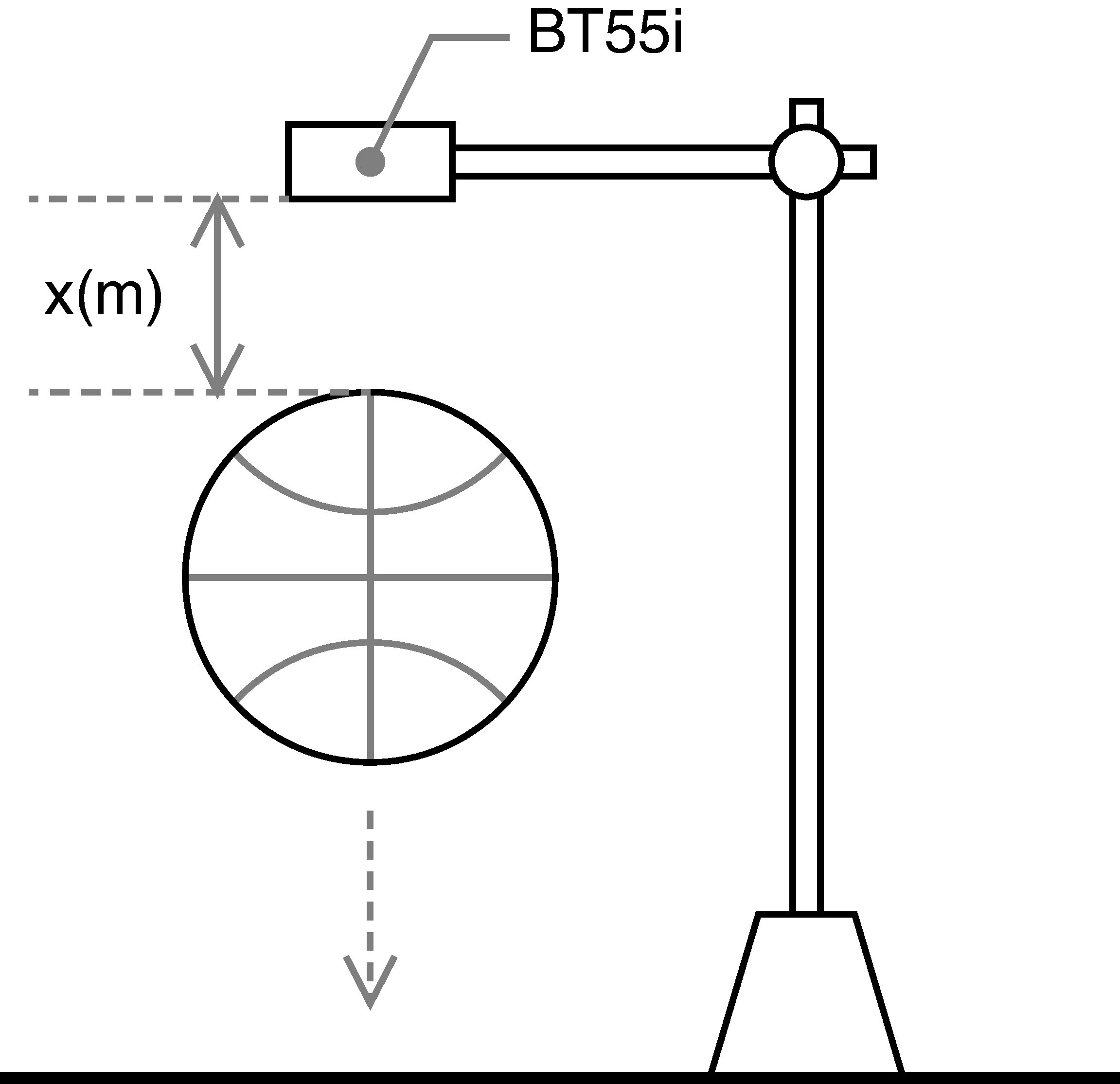
Measuring Ball Bouncing and Analyzing the Data with Ball Bounce
-
Prepare for measurement.
-
Set up the experimental equipment and attach the motion sensor to it.
-
Use the cable to connect the calculator to CLAB, and then turn on CLAB.
-
Turn on the calculator, and then start the E-CON5 app.
-
Connect the motion sensor to CLAB sensor terminal 1.
-
Configure measurement method settings.
-
Highlight the first row of the top screen and press O.
-
On the Setup menu that appears, select [Measurement Method].
-
On the Measurement Method screen that appears, configure settings as shown here.
-
Press b to return to the top screen.
-
Perform the measurement.
-
On the top screen, highlight
, and then press O. -
Hold the ball directly under the motion sensor.
-
Press O to start the measurement, and immediately release the ball.
-
Process the measurement data using Ball Bounce.
-
Select T > [Display Table] to display the measurement results on the table screen.
-
Select T > [Advanced Function] > [Ball Bounce].
-
Select [Yes].
-
Select [OK].
-
Enter the ball’s weight in kilograms, and then press O.
-
Switch on (
) the graph(s) you want to display. -
Highlight
, and then press O. -
Use the Statistics app to draw graphs.
-
Select h > Statistics to start the Statistics app.
-
Press > to go to the Setup tab.
-
Highlight
 , and then press O.
 -
Press b to return to the Draw Statistics Graph menu on the Setup tab.
-
Change the draw settings of Graph2 and Graph3 to None.
-
Highlight
, and then press O.
Important!
The motion sensor must be connected to sensor terminal 1. Ball Bounce processes measurement data from CH1.
CLAB: Connected
Type: Time-based
Unit: sec, /sec
Duration: 5 s
Frequency: 30 /s
Samples: 151
Trigger: [OK]
This causes the measurement standby screen to appear. Measurement will start when you press O in step (3), below.
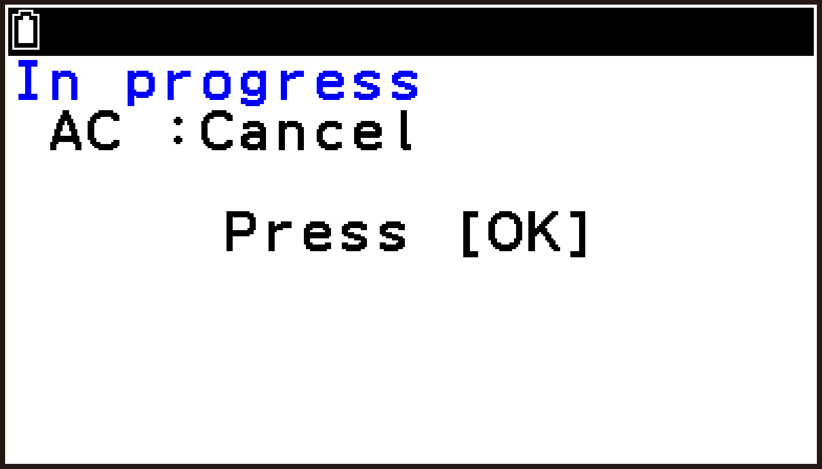
The ball will fall and bounce on the floor several times.
While measurement is in progress, measured values appear in real time on the graph. During measurement, measured values appear in real time on the graph.
After 5 seconds, the measurement ends automatically, and the graph screen (Analysis tab) appears.
X-axis (t(s)): Elapsed time (seconds) from the start of measurement
Y-axis (x(m)): Distance (m) from the sensor to the ball
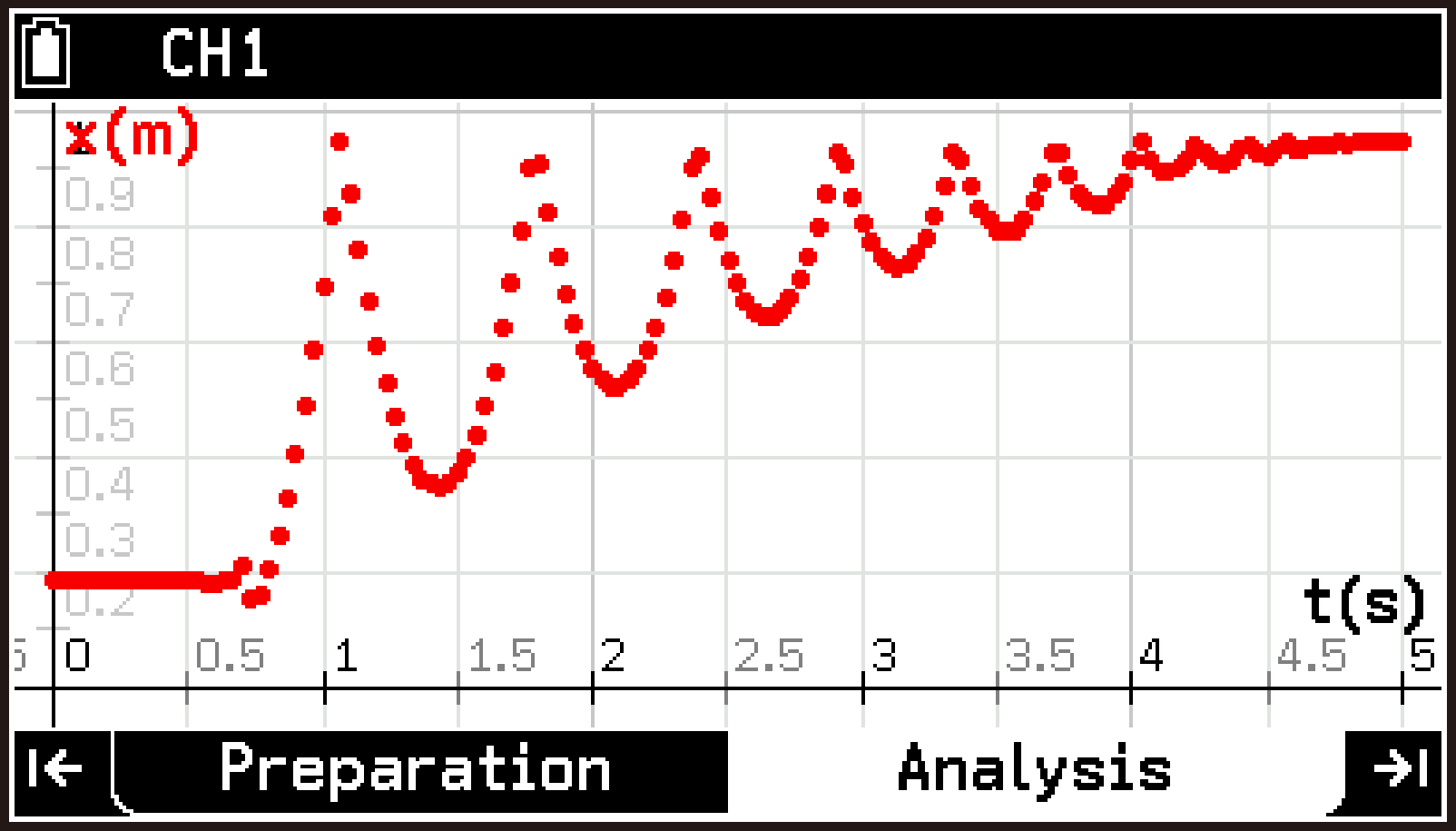
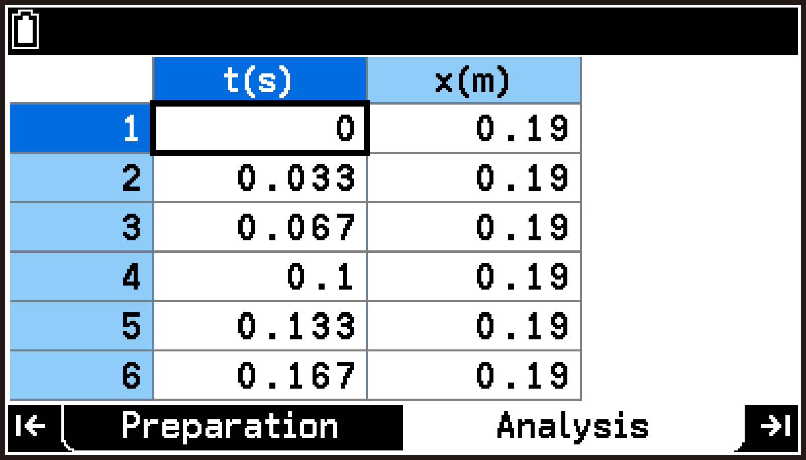
A message appears asking you to confirm that the data was collected using CH1.
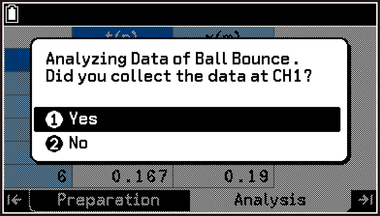
A warning dialog appears explaining that Statistics app settings will be changed.
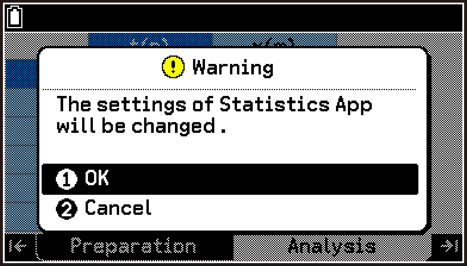
Important!
Selecting [OK] on the warning dialog, the contents of List 1 through List 9 will be overwritten, and graph drawing settings of the Statistics app will be changed automatically.
This displays a dialog for entering the weight of the ball.
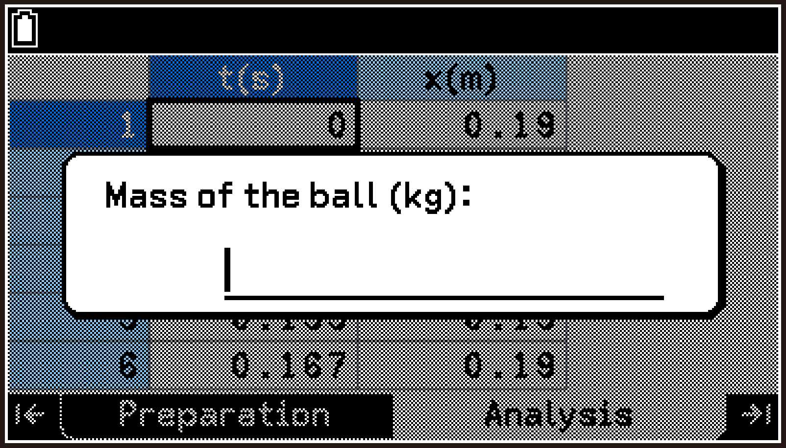
This displays the Select Graph dialog. On this dialog, select the graphs to be displayed using the Statistics app.
Distance: Time–distance graph
Velocity: Time–velocity graph
Acceleration: Time–acceleration graph
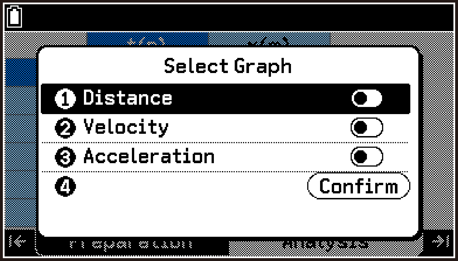
Attempting to continue without switching on at least one graph causes the error message “No item is selected” to appear. Be sure to switch at least one graph.
This displays the Next Tasks dialog.
List 1 and List 2 are overwritten with the measurement data, and List 3 through List 9 are overwritten with data calculated from the measurement data graph drawing settings of the Statistics app are also changed automatically.
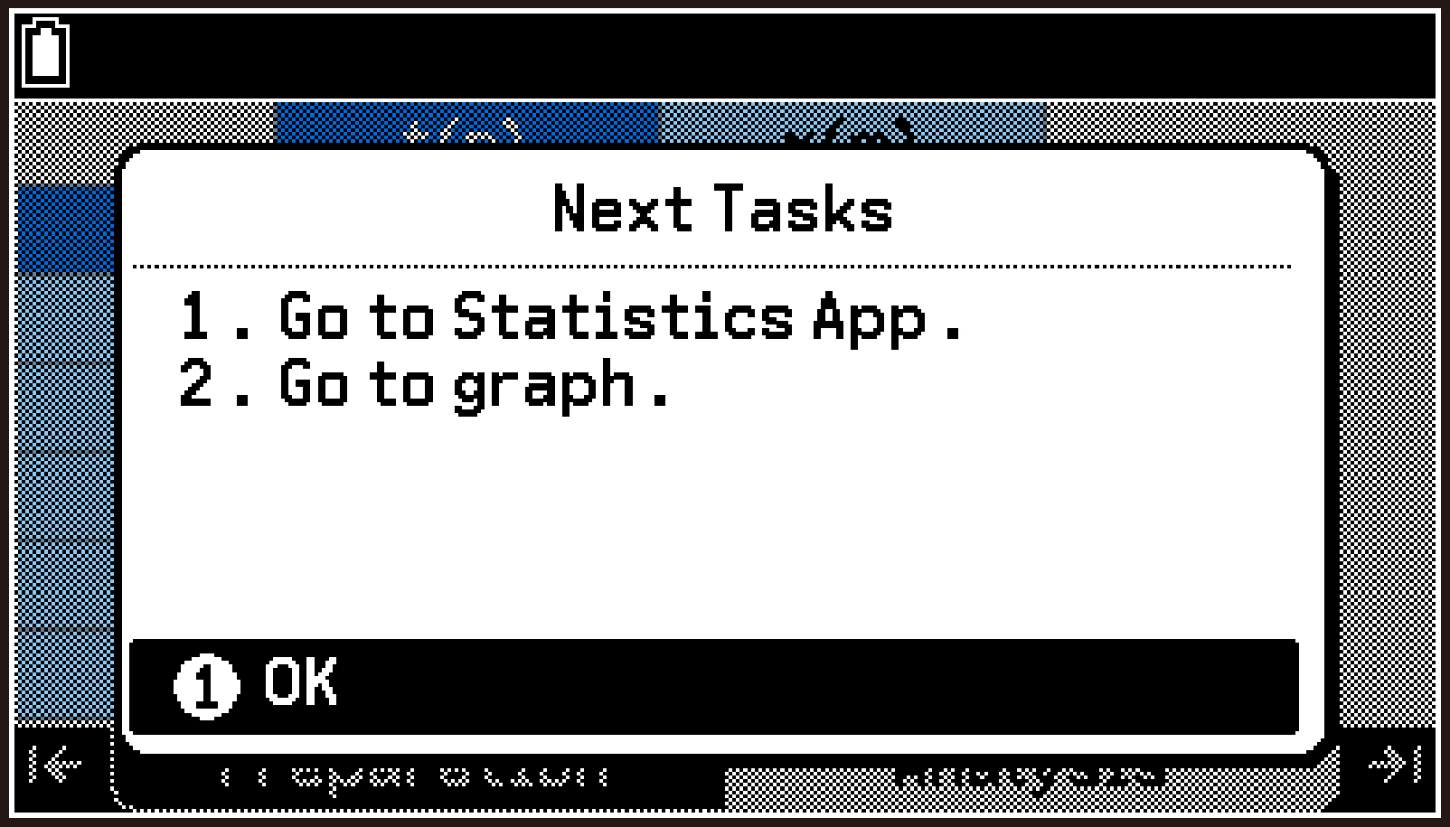
The List Editor shows the data output from the E-CON5 app.
For details about the output data, see List of Data Output to List Variables.
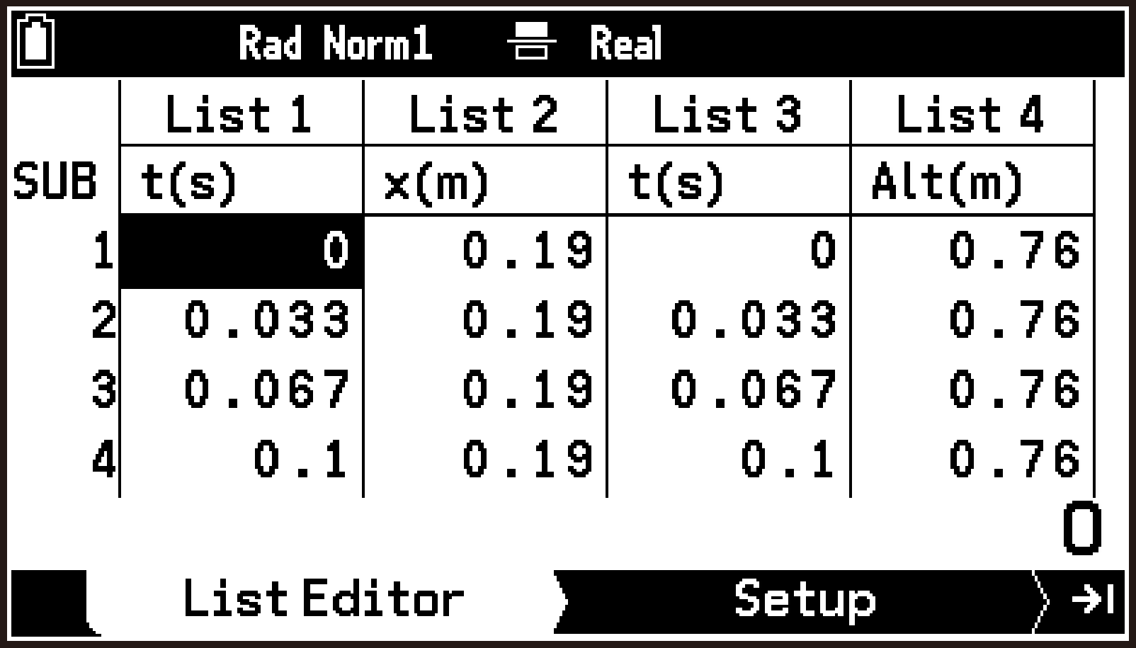
Confirm that the Draw Statistics Graph menu appears on the Setup tab as shown to the right. Graph1 through Graph3 are assigned automatically to the following graphs (if you switched on all graphs in step 4-(6)).
Graph1: Time–distance graph
Graph2: Time–velocity graph
Graph3: Time–acceleration graph
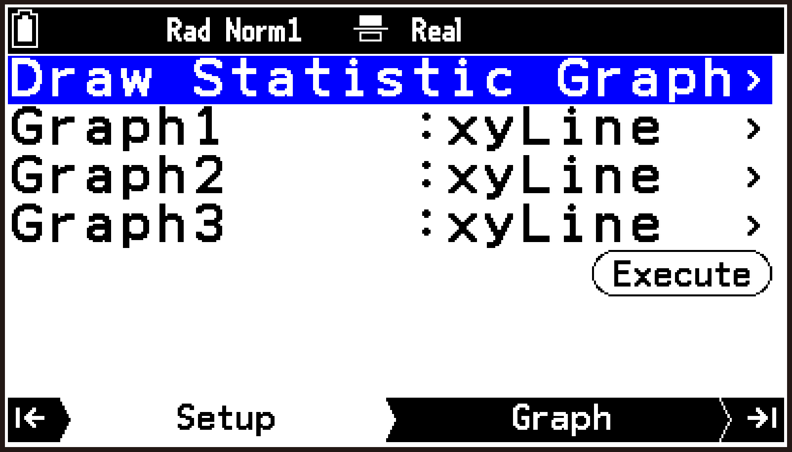
This draws all the graphs you switched on in step 4-(6).
In steps (4) through (6) below, you select and draw only one graph.
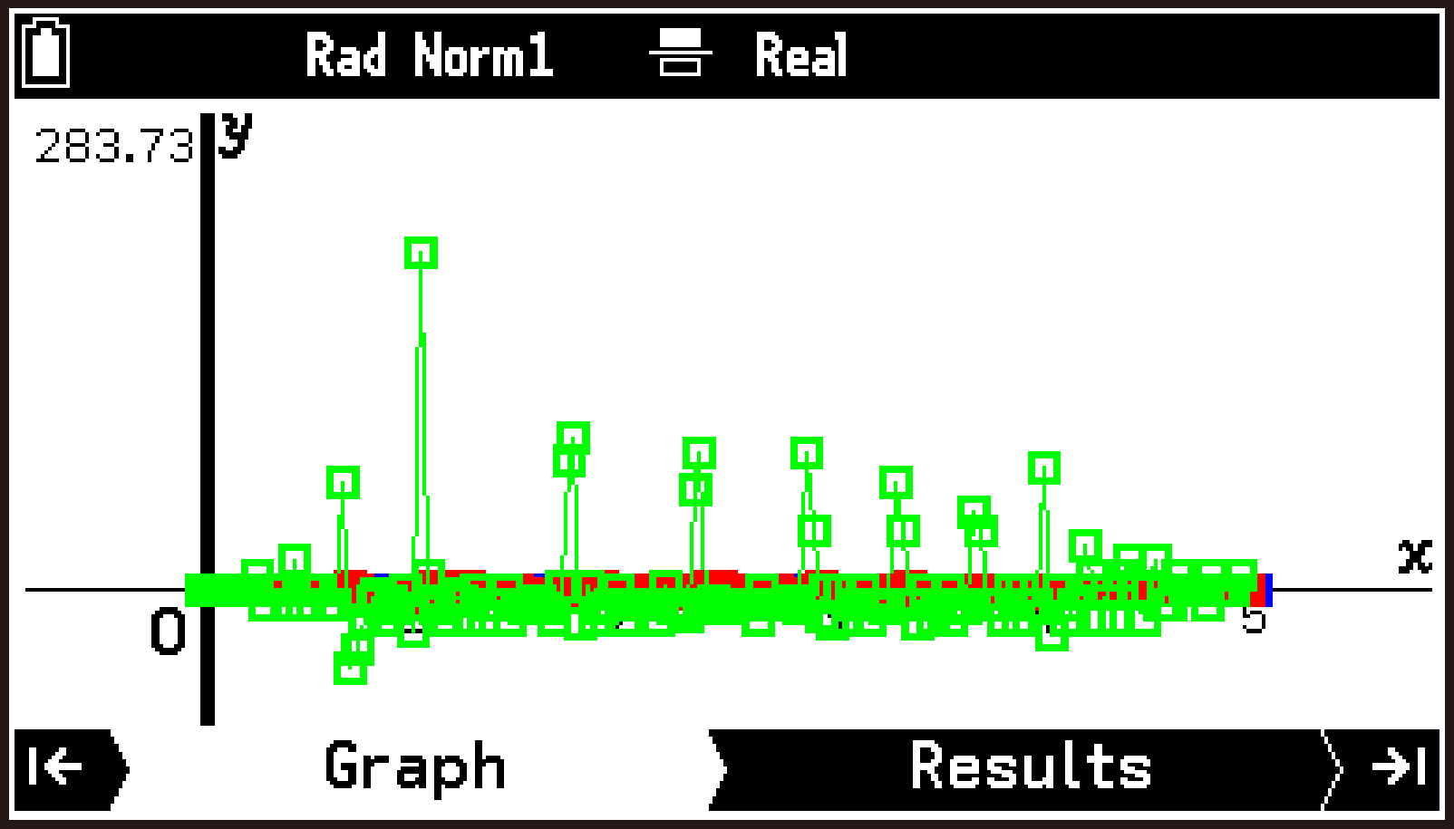
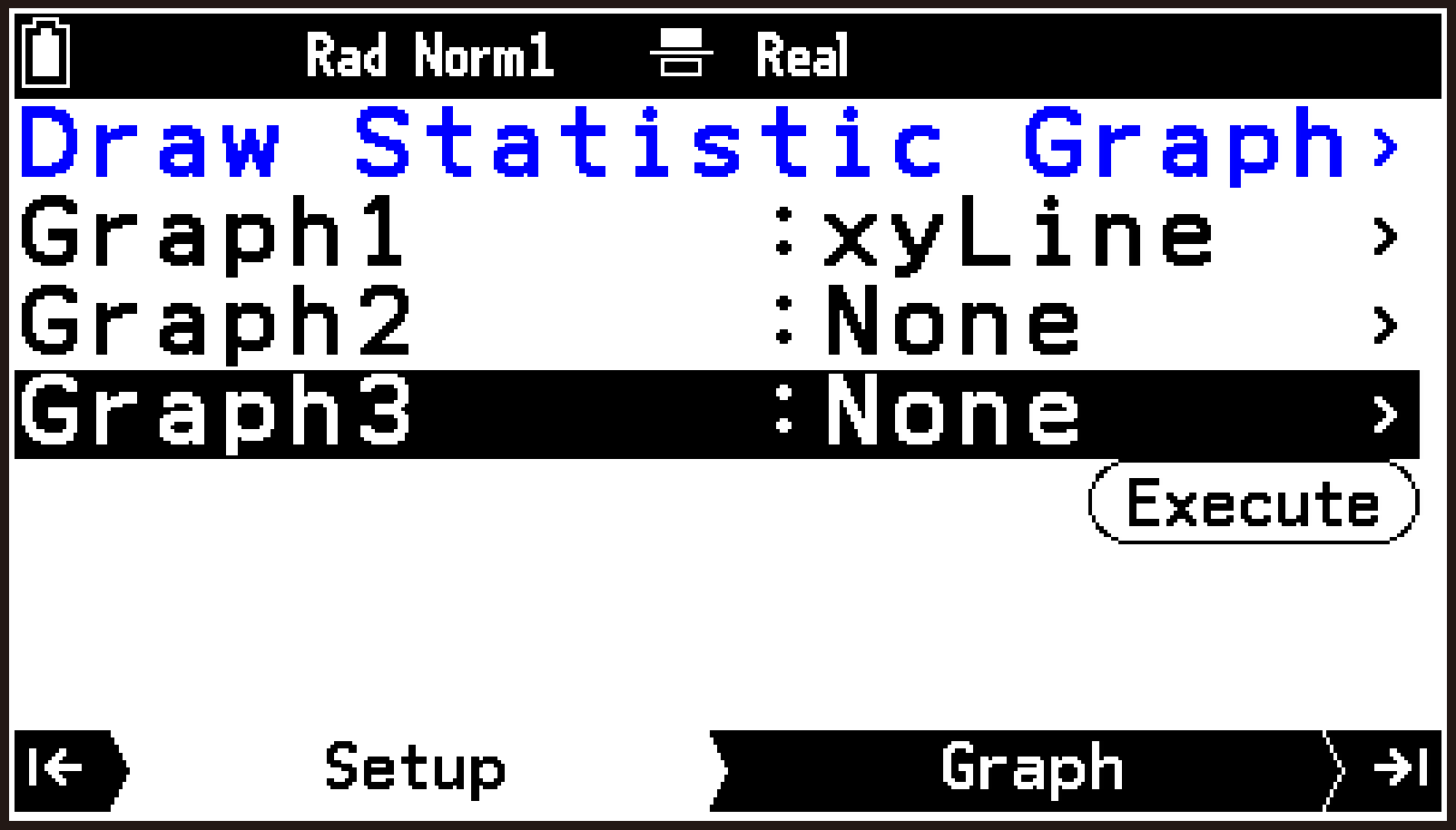
This draws Graph1 only. You can also draw Graph2 only and Graph3 only the same way.
When analyzing data, it is convenient to use the graphs drawn individually. For details about graph analysis operations, see the Statistics app section of this manual.
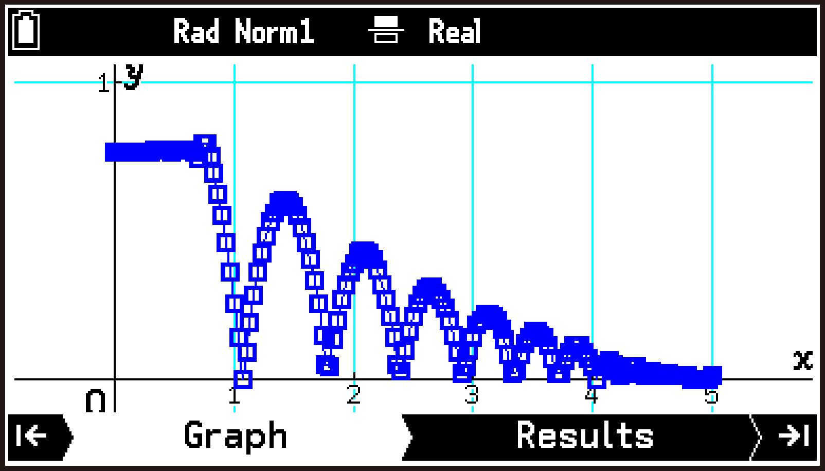
List of Data Output to List Variables
The data output to list variables by Ball Bounce is shown in the following table.
|
List Name |
Sub-name |
Data |
|---|---|---|
|
List 1 |
t(s) |
Raw time data measured by CLAB. |
|
List 2 |
x(m) |
Raw distance data measured by CLAB. |
|
List 3 |
t(s) |
Time data corrected for analysis based on List 1, used for calculations in Lists 4 through 9. In most cases, each element in List 3 is identical to the corresponding element in List 1. |
|
List 4 |
Alt(m) |
Distance from the floor to the ball. Calculated as , where is the distance measured by CLAB (sensor to ball) and is the maximum value of . |
|
List 5 |
v(m/s) |
Ball velocity. Calculation is performed based on List 3 and List 4 data. |
|
List 6 |
a(m/s2) |
Ball acceleration. Calculation is performed based on List 3 and List 5 data. |
|
List 7 |
Ep(J) |
Ball potential energy. Calculated from the data in List 4 (××List 4).* |
|
List 8 |
Ec(J) |
Ball kinetic energy. Calculated from the data in List 5 (1/2××(List 5)2).* |
|
List 9 |
EM(J) |
Ball mechanical energy. Calculated from the data in Lists 7 and 8 (List 7 + List 8). |
: Ball weight entered with the E-CON5 app, : gravitational acceleration
Operation Flow According to Measurement Method
This section explains the overall flow of operations for the following measurement methods using the E-CON5 app.
Measuring in Connected Mode Using the Time-based Type
Measuring in Connected Mode Using Manual Type
Measuring in Connected Mode Using Interval Type
Measuring with Standalone Mode
Measurement Using a Saved Setup
This section provides only simplified, typical steps for each measurement method. For details about each operation or setting, see the individual explanations in this chapter.
Measuring in Connected Mode Using the Time-based Type
-
Use the cable to connect the calculator to CLAB, and then turn on CLAB.
-
Turn on the calculator, and then start the E-CON5 app.
-
Connect the sensors to be used for measurement to CLAB sensor terminals 1, 2, and 3.
-
Highlight the channel(s) to which the sensor(s) is connected (CH1, CH2, or CH3).
-
Select T > [Sensor Menu] > [Library].
-
Select the applicable sensor(s) from the library screen that appears.
-
Enable the CLAB built-in accelerometer if required.
-
Highlight the first row of the top screen and press O.
-
From the menu that appears, select [Accelerometer], and switch [A-X], [A-Y], and [A-Z] to enabled (
). -
Confirm that the sensors to be used for measurement are shown on the top screen.
-
Configure measurement method settings.
-
Highlight the first row of the top screen and press O.
-
On the Setup menu that appears, select [Measurement Method].
-
On the Measurement Method screen that appears, configure the following settings.
-
To complete the setting procedure and return to the top screen, press b.
-
To start measurement, highlight
, and then press O. -
Display and analyze the collected data in various formats.
-
Save the measurement data to a list variable or a CSV file, if required.
-
Save the setup for this measurement if required.
For details about the cable used for connection, see Connecting the Calculator and CLAB.
When communication between the calculator and CLAB is established, the status of each channel appears on the top screen of the E-CON5 app.
If the message “CLAB disconnected” appears on the top screen, it means there is a communication problem between the calculator and CLAB. If this happens, check to make sure both ends of the cable are firmly inserted into the calculator and CLAB jacks.
When a sensor is auto-recognized, its measurement value appears on the top screen.
If a sensor is not auto-recognized, select it from the library using the following steps.
Use d or u to scroll and check the active sensors.
CLAB: Connected
Type: Time-based
Unit: sec, /sec
Duration: Specifies the measurement time (Initial Default: 10 seconds).
Frequency: Inputs the desired sampling frequency (Initial Default: Once/second).
Samples: Automatically adjusted according to the input values for Duration and Frequency above (Initial Default: 11).
Trigger: None
For details about each setting item, see Time-based Type Setting Items.
This starts measurement. During measurement, values are displayed in real time on the graph.*
To interrupt measurement, press a.
If you are measuring on multiple channels simultaneously, use U or D to switch between graphs.
Measurement ends automatically and the graph screen (Analysis tab) appears when the specified time elapses.
On the graph screen, select T > [Display Table] to display the table screen.
On the graph screen, select T > [Analyze Graph]. Next, choose an analysis tool from the menu that appears. See Graph Analysis (Analysis Tab).
See Saving Measurement Data (Analysis Tab).
If a high sampling frequency is specified, the graph is not displayed in real time. Instead, the progress of data being downloaded from CLAB to the calculator is shown. When the download is complete, the graph screen (Analysis tab) appears.
Important!
If you specify a long measurement time (Duration) in step 6-(3), check the remaining battery power of the calculator before performing a measurement. If the remaining battery power is insufficient, the battery may run out before the specified measurement time elapses, causing the calculator to turn off automatically and the measurement to be interrupted.
Measuring in Connected Mode Using Manual Type
-
Perform steps 1 through 5 of the procedure under Measuring in Connected Mode Using the Time-based Type.
-
Configure measurement method settings.
-
Highlight the first row of the top screen, and then press O.
-
On the Setup menu that appears, select [Measurement Method].
-
On the Measurement Method screen that appears, configure the following settings.
-
To complete the setting procedure and return to the top screen, press b.
-
To start measurement, highlight
, and then press O. -
Perform the procedure under Measuring in Connected Mode Using the Time-based Type starting from step 8.
CLAB: Connected
Type: Manual
Samples: Specifies the number of samples (Initial Default: 10).
Input: Specifies, by selecting 1 Entry, 2 Entries, or 3 Entries, how many values are to be entered manually for each measurement. For example, to measure gas pressure with a pressure sensor connected to CLAB and manually enter the corresponding volume obtained separately, select 1 Entry.
If no manual input is required, select None (initial default).
Quantity, Unit, Digits: These settings specify the quantity symbol, unit, and number of decimal places for each manually entered value specified under Input.
For details about each setting item, see Manual Type Setting Items.
This starts measurement. Each press of O collects a data sample and displays the measurement value on the graph in real time.
If you selected an option other than None under Input in step 2-(3), a dialog for entering values appears each time you press O (one, two, or three times, depending on the number of inputs you specified). Enter a value in each input dialog, and then press O to proceed to the next dialog.
To interrupt measurement, press a.
When collection of the specified number of samples is complete, the measurement ends and the graph screen (Analysis tab) appears.
Measuring in Connected Mode Using Interval Type
Important!
When measuring with the Interval type, you can use only one sensor as the signal source for time-interval measurement. Generally speaking, be sure to use an analog-range sensor, and do not use a counter-range sensor.
As exceptions to the above, CMA photogates (BT63i, 0663i) and CMA radiation sensors (0666i, BT70i) can be used as signal sources for time-interval measurement. When these sensors are connected to CLAB and auto-recognized, their counter range is shown in the sensor details dialog. However, for time-interval measurement, the analog range of 0 to 5 V and a threshold of 2.5 V are applied.
-
Perform steps 1 through 5 of the procedure under Measuring in Connected Mode Using the Time-based Type.
-
Configure measurement method settings.
-
Highlight the first row of the top screen, and then press O.
-
On the Setup menu that appears, select [Measurement Method].
-
On the Measurement Method screen that appears, configure the following settings.
-
To complete the setting procedure and return to the top screen, press b.
-
To start measurement, highlight
, and then press O. -
Perform the procedure under Measuring in Connected Mode Using the Time-based Type starting from step 8.
CLAB: Connected
Type: Interval
Samples: Inputs the number of samples (Initial Default: 10).
Source: Specifies the channel (CH1, CH2, CH3) to which the sensor used as the signal source is connected.
Threshold: Enter the value you want to specify as the signal threshold. The initial default value is 50% of the measurement range of the sensor being used as the signal source.
Flank: Select the combination of the start and end points of the time interval (Rise-Rise, Fall-Fall, Rise-Fall, Fall-Rise, Both). Select the setting that is appropriate for the measurement target.
Repeat: Off (For operation when On, see “Note” below.)
For details about each setting item, see Interval Type Setting Items.
This starts measurement, and the message “Waiting for sample...” appears in the lower left of the screen. It remains there until the first signal matching the Threshold and Flank settings is detected from the sensor connected to the source channel. After detection, measurement values are displayed on the graph in real time. The vertical axis of the graph shows the measured time interval (Δt(s)), while the horizontal axis shows the index (n).
To interrupt measurement, press a.
When collection of the specified number of samples is complete, the measurement ends and the graph screen (Analysis tab) appears.
Note
If you selected On for Repeat in step 2-(3) above, the dialog “Repeat measurement?” appears when collection of the specified number of samples is complete.
Selecting [Yes] on this dialog causes measurement to continue until the specified number of samples is collected again. Select [No] on this dialog to end measurement.
Measuring with Standalone Mode
-
Perform steps 1 through 5 of the procedure under Measuring in Connected Mode Using the Time-based Type.
-
Configure measurement method settings.
-
Highlight the first row of the top screen, and then press O.
-
On the Setup menu that appears, select [Measurement Method].
-
On the Measurement Method screen that appears, configure settings as shown here.
-
To complete the setting procedure and return to the top screen, press b.
-
To start measurement, highlight
, and then press O. -
Select [Send Setup to CLAB.].
-
To return to the top screen from the Uploaded screen, press O.
-
Disconnect the cable from the calculator and CLAB.
-
To start measurement, press the CLAB power button.
-
Use the cable to re-connect the calculator to CLAB.
-
On the E-CON5 top screen, highlight
, and then press O. -
Select [Get measured data.].
-
Perform the procedure under Measuring in Connected Mode Using the Time-based Type starting from step 8.
CLAB: Standalone
Unit: sec, /sec
Duration: Specifies the measurement time (Initial Default: 10 seconds).
Frequency: Inputs the desired sampling frequency (Initial Default: Once/second).
Samples: Automatically adjusted according to the input values for Duration and Frequency above (Initial Default: 11).
Trigger: CLAB button (Measurement starts when you press the CLAB power button.)
For details about each setting item, see Time-based Type Setting Items.
This displays a dialog like the one to the right.
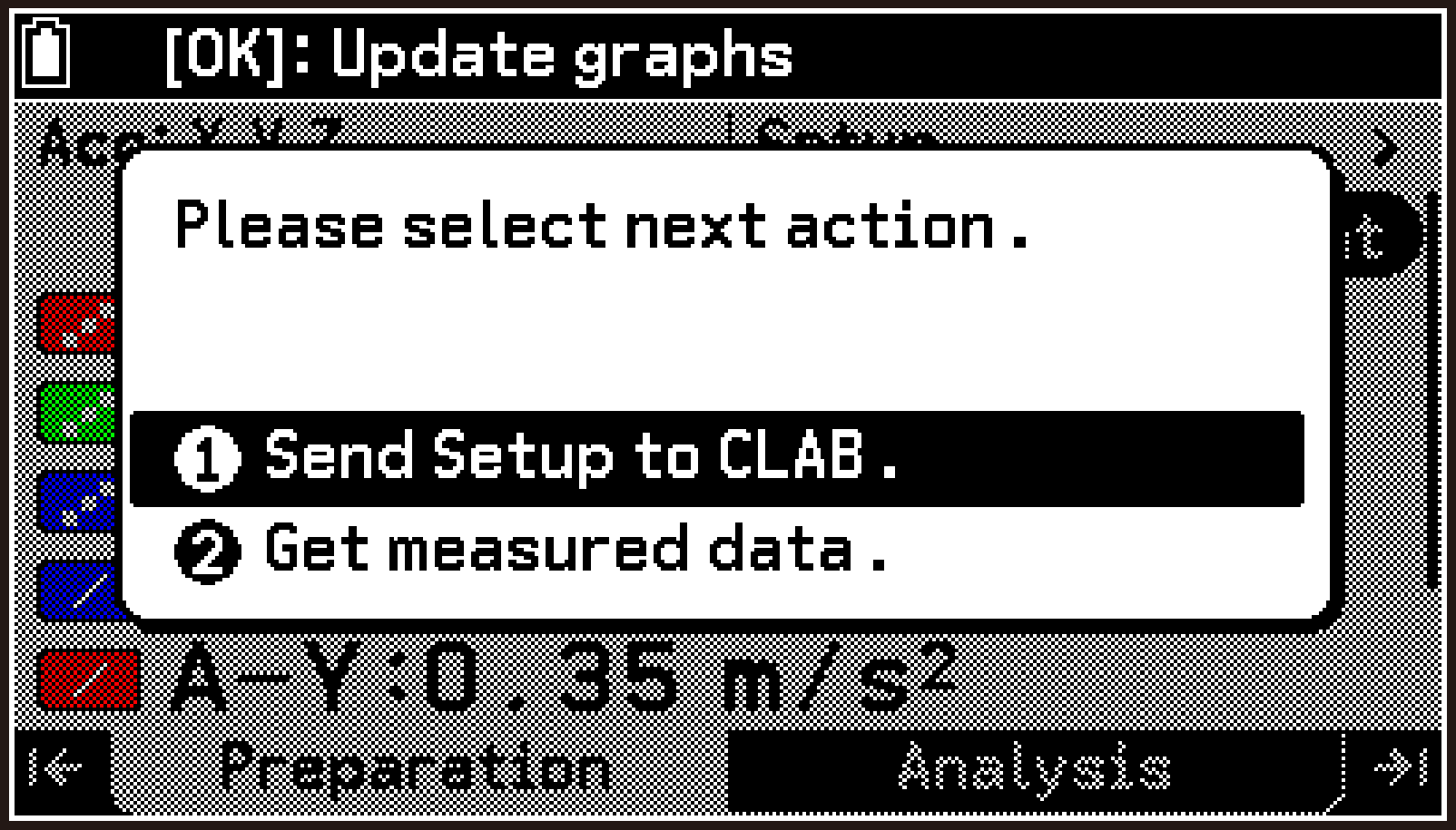
After the setup is uploaded from the E-CON5 app to CLAB, the screen switches to Uploaded.
The LED on the right half of the CLAB power button lights blue, indicating that CLAB is in measurement standby.
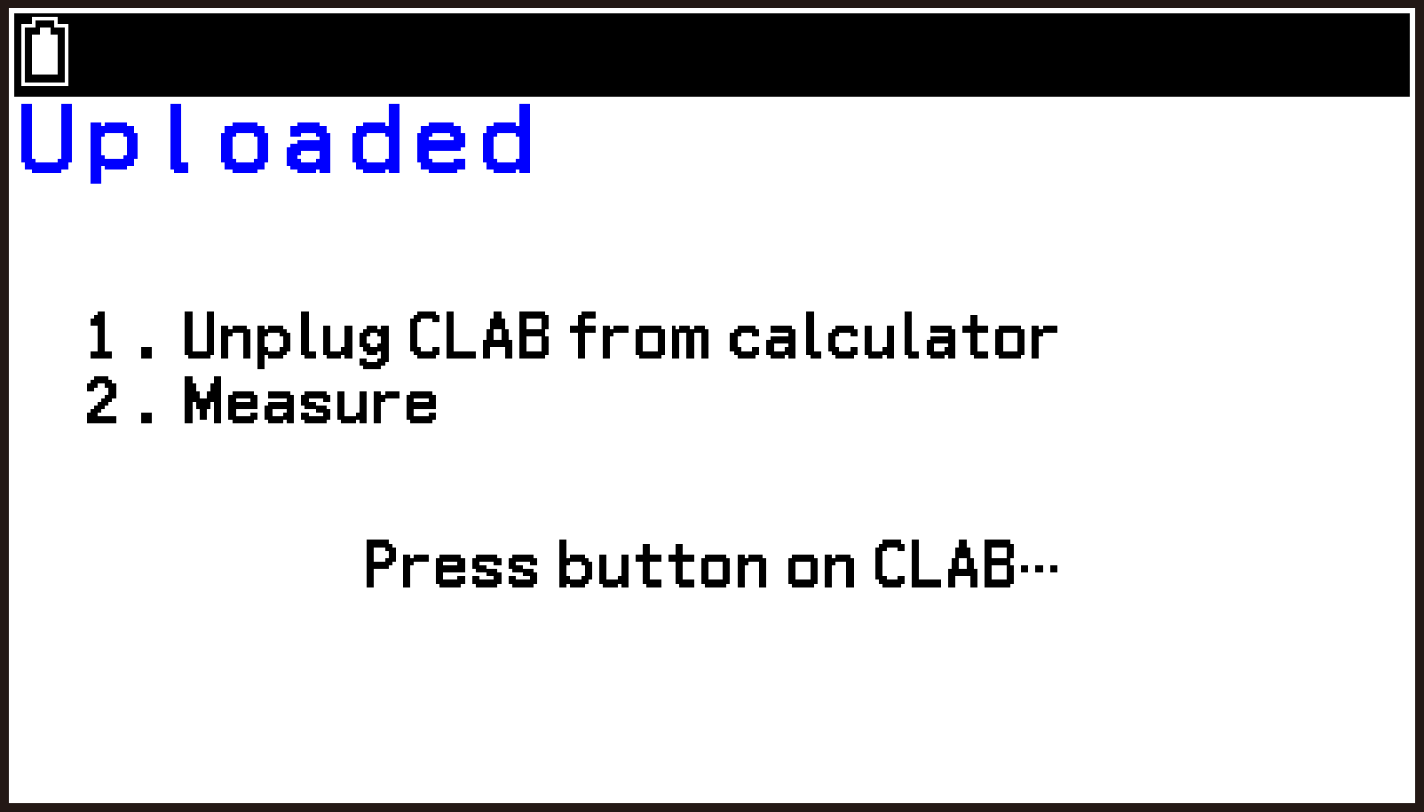
Until you start measurement in step 7, you may, if necessary, turn off CLAB. When you turn CLAB back on, the LED on the right half of the power button lights blue, indicating that CLAB is in measurement standby.
Until you reconnect the calculator and CLAB in step 8, you may use other apps on the calculator or even turn the calculator off. However, do not perform any of the operations below. If you do, you will not be able to download measurement data stored in CLAB to the calculator.
Resetting calculator main memory with the System app
Changing the CLAB operation mode to Connected with the E-CON5 app
During measurement, the LED on the right half of the CLAB power button flashes green.
To interrupt measurement, press the CLAB power button.
Measurement ends automatically after the specified duration elapses. At this time, the LED on the right half of the CLAB power button lights green, indicating that measurement data is saved in CLAB memory.
This displays the same dialog box as that in step 3.
This downloads the measurement data from CLAB to the calculator, and displays the graph screen (Analysis tab).
Measurement Using a Saved Setup
-
Perform steps 1 and 2 under Measuring in Connected Mode Using the Time-based Type.
-
Recall the setup you want to use for measurement.
-
Highlight the first row of the top screen, and then press O.
-
On the menu that appears, select [Setup Memory].
-
Use d and u to highlight the file whose setup you want to use for measurement.
-
To recall a setup, select T > [Open Memory].
-
On the confirmation dialog that appears, select [OK].
-
Press b to return to the top screen.
-
Connect the sensor(s) you specified with the setup to CLAB sensor terminals 1, 2, and/or 3.
-
Start measurement.
If necessary, you can select T > [Information] to display a setup information dialog and check setup details. To close the dialog, press O.
You can view the sensor specified by the setup on the top screen or in the sensor details dialog for each channel.
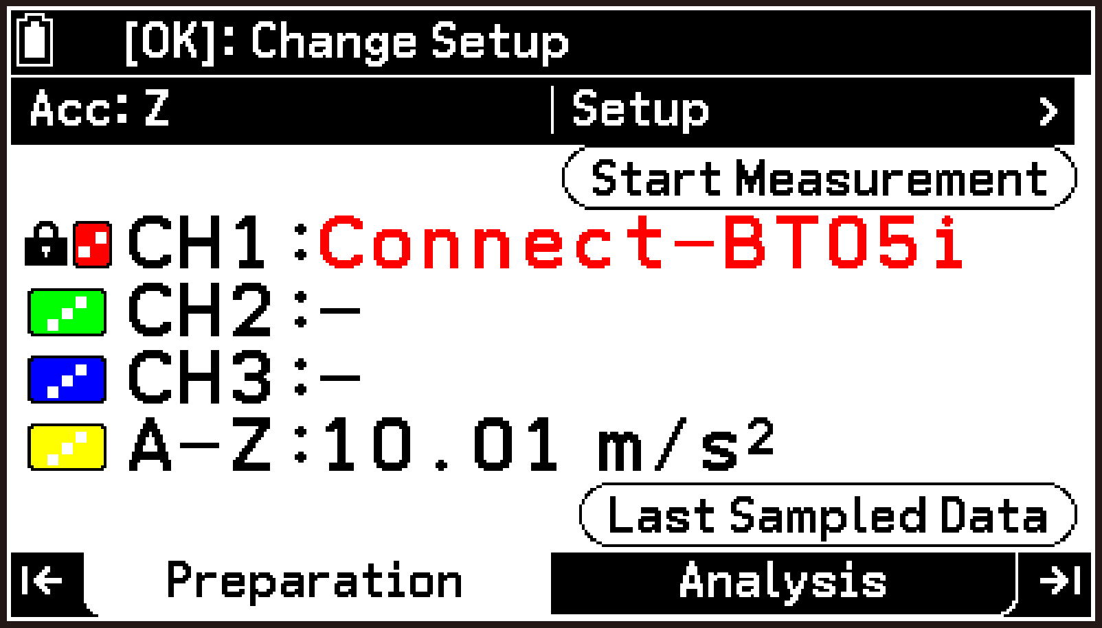
Top screen
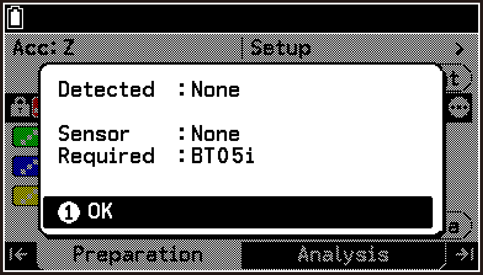
Sensor details dialog
For information about starting a measurement and subsequent operations, see the appropriate sections below for each measurement type.
Procedure under Measuring in Connected Mode Using the Time-based Type starting from step 7.
Procedure under Measuring in Connected Mode Using Manual Type starting from step 3.
Procedure under Measuring in Connected Mode Using Interval Type starting from step 3.
E-CON5 Application Error Messages
|
Message |
Meaning |
Required Action |
|---|---|---|
|
CLAB is not connected. |
You attempted to perform an operation that requires the calculator to be connected to CLAB (for example, trying to display CLAB version information when CLAB is not connected). |
Connect the calculator to CLAB, and then turn on CLAB. Make sure both cable plugs are firmly inserted into the calculator and CLAB jacks. |
|
Measurement is interrupted. |
Measurement was interrupted because you pressed a during measurement in Connected mode. Measurement was interrupted because the connection between the calculator and CLAB was interrupted during Connected mode measurement with the Manual type. |
To save the measurement data collected up to the point of interruption, select [Yes]. If you do not need the data, select [No]. If measurement was interrupted unintentionally, check the connection between the calculator and CLAB, and then try to perform the measurement again. |
|
Data Reading ERROR |
The connection between the calculator and CLAB was lost during Connected mode measurement with the Time-based type, causing transfer of measurement data to be interrupted. |
Check the connection between the calculator and CLAB, and then try to perform the measurement again. |
|
Can’t save file. |
A setup could not be saved to a file. |
Check for the following: Are there any issues with Measurement Method screen settings? Is there sufficient storage memory remaining? |
|
Can’t save sensor. |
A custom sensor could not be saved to a file. |
Check for the following: Are there any issues with Properties screen settings? Is there sufficient storage memory remaining? |
|
Invalid Type |
You tried to open a setup file or view its information, but the contents of the file were invalid. You tried to assign a custom sensor file to a channel or edit the file, but the contents of the file were invalid. |
Even if the file name extension is .s4t, you cannot use a file unless its contents are a setup. Use a correct file. Even if the file name extension is .s4n, you cannot use a file unless its contents are a custom sensor. Use a correct file. |
|
Nothing to measure |
You tried to start a Time-based type or Interval type measurement, but no sensor was connected. |
Correctly connect the sensor you want to use for measurement to CLAB, and then start measurement. |
|
Nothing to measure |
You tried to start a Manual type measurement, but no sensor was connected. You did not manually enter data when manual data entry was required. |
Correctly connect the sensor you want to use for measurement to CLAB, and then start measurement. Manually enter data when the manual input prompt dialog appears during measurement. |
|
No interval source specified. |
You tied to start an Interval type measurement, but left the Source setting on the Measurement Method screen as “None”. |
Select a Source before starting measurement. |
|
Unavailable interval source. |
You tried to start an Interval type measurement without connecting the sensor to be used as the signal source. You did not specify a sensor as the signal source. |
Specify the sensor to be used as the signal source, connect the sensor to CLAB, and then start measurement. |
|
Calibration failed. |
Calibration failed because CLAB was turned off or the cable connecting the calculator and CLAB was disconnected during calibration. |
Check the connection between the calculator and CLAB, and redo calibration from the beginning. Also check to make sure the calculator battery level and the CLAB charge level are sufficient. |
|
Nothing to download. |
Following Standalone mode measurement, you tried to connect the calculator and CLAB to download measurement data from CLAB, but there was no measurement data in CLAB memory. |
Possible causes for this include disconnection of the sensor used for measurement from CLAB, or a sensor malfunction that prevented data collection. Check the following: Is the sensor correctly connected to CLAB? Do measurement values from the sensor appear on the E-CON5 app top screen while CLAB is connected to the calculator? |
|
Measurement ERROR |
Following Standalone mode measurement, you tried to connect the calculator and CLAB and download measurement data from CLAB, but some invalid operation (pressing h, cable disconnection, etc.) occurred during data transfer. |
Try the operations starting from step 8 of the procedure under Measuring with Standalone Mode. However, if this does not cause the “Please select next action.” dialog to appear, or if the dialog does appear but selecting [Get measured data.] results in an error, perform the measurement again. |
|
Screen Receiver Mode! |
You tried to delete a setup file or custom sensor file while the calculator was connected to a computer with its screen displayed on Screen Receiver. |
Disconnect from Screen Receiver before deleting the file. |
Appendix
E-CON5 App Limitations
The maximum values for measurement time, sampling frequency, and number of samples that can be specified with the E-CON5 app are shown in the following table.
|
Setting Item |
Upper Specification Limit |
|---|---|
|
Duration (measurement time) |
162,000 seconds (45 hours) |
|
Frequency (sampling frequency) |
1 sensor: 100,000/s 2 sensors: 50,000/s 3 sensors: 15,000/s 1 BT55i sensor: 100/s 2 BT55i sensors: 20/s 3 BT55i sensors: 5/s Sensor with count function: 2,500/s Pitch sensor: 100/s CLAB built-in accelerometer: 800/s |
|
Samples (number of samples) |
30,000 |
The upper limits above are the possible values for each individual setting item. Based on the values specified for two of the three items, the remaining setting value is adjusted. For example, when measuring with one sensor, if you specify the maximum sampling frequency (100,000/s) and the maximum number of samples (30,000), the measurement time is automatically set to 0.3 seconds (30,000 ÷ 100,000). (On the Measurement Method screen, the actual display will be 0.2999 s.)
Also, if the setup of the sensor at the time measurement is started differs from the setting values currently configured on the Measurement Method screen, a warning dialog will appear and the setting values will be adjusted automatically.
Example: When only a voltage sensor is connected, the sampling frequency is set to 1,000/s, and then the built-in accelerometer of CLAB is enabled before starting measurement. In this case, since the maximum sampling frequency that can be specified for the built-in accelerometer is 800/s, a warning dialog like the one shown here will appear.
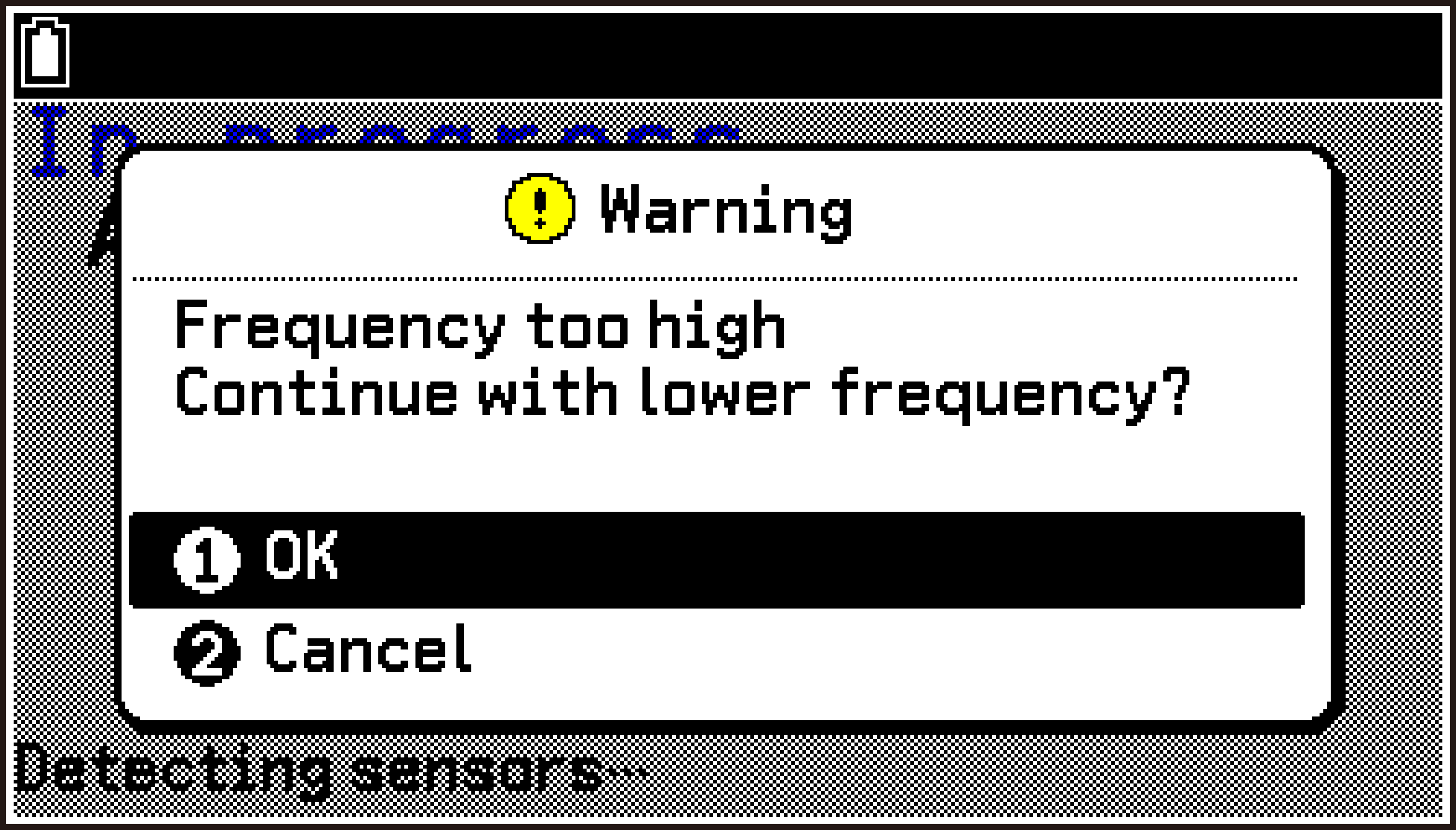
If you select [OK], the sampling frequency is automatically adjusted (in this case changed to 800/s), and measurement starts.
Important!
Continuous measurement performed for an extended period may cause the battery to run out more quickly than usual.
When performing long-term measurement, keep an eye on the remaining battery power of the calculator. If the remaining battery power is insufficient, the battery may run out before the specified measurement time elapses, causing the calculator to turn off automatically and the measurement to be interrupted.
Real-time Display of Measurement Data During Measurement
Whenever possible, the E-CON5 app displays measurement data in real time as a graph during measurement execution.
The following are guidelines for when graphs can be displayed in real time.
Measuring with one sensor: Sampling frequency setting* within 400/s
Measuring with two sensors: Sampling frequency setting* within 200/s
Measuring with three sensors: Sampling frequency setting* within 100/s
Frequency setting of the Measurement Method screen
If the E-CON5 app cannot display measurement data in real time as a graph, the following screen appears when measurement starts.
In this case, the graph screen based on the measured values will be displayed after measurement is complete.
E-CON5 App Data Storage
Various types of E-CON5 app data (such as setup data and measurement results) are stored in the calculator’s main memory and storage memory. For details about main memory and storage memory, see Memory App.
Main Memory
Within the E-CON5 group in the calculator’s main memory, the information configured with the Measurement Method screen and the latest measurement data are stored. The names and content of the data saved in the E-CON5 group are shown in the following table.
|
Data Name |
Contents |
|---|---|
|
|
Data of sensors automatically recognized (or manually assigned) on channels CH1, CH2, and CH3. |
|
|
Sensor data when the -axis, -axis, and -axis of the accelerometer are enabled. |
|
|
Acceleration sensor -axis, -axis, -axis measurement data. |
|
|
Measurement data of sensors connected to CH1, CH2, CH3. |
|
|
Graph data resulting from creation of custom graphs (Custom 1, Custom 2, Custom 3). |
|
|
Measurement data when the measurement type is Manual. |
|
|
Data that retains sensor measurement values adjusted (calibrated) using Edit Value. |
|
|
Setup data created when settings are changed on the Measurement Method screen. |
|
|
Measurement result data that is automatically updated each time a measurement is completed. For measurements with an extremely large number of samples, this data is not created. Instead, a file named sample.dat is created directly under the E-CON5 folder in storage memory. |
Storage Memory
Files of the E-CON5 app are stored in the calculator’s storage memory under the following hierarchy.
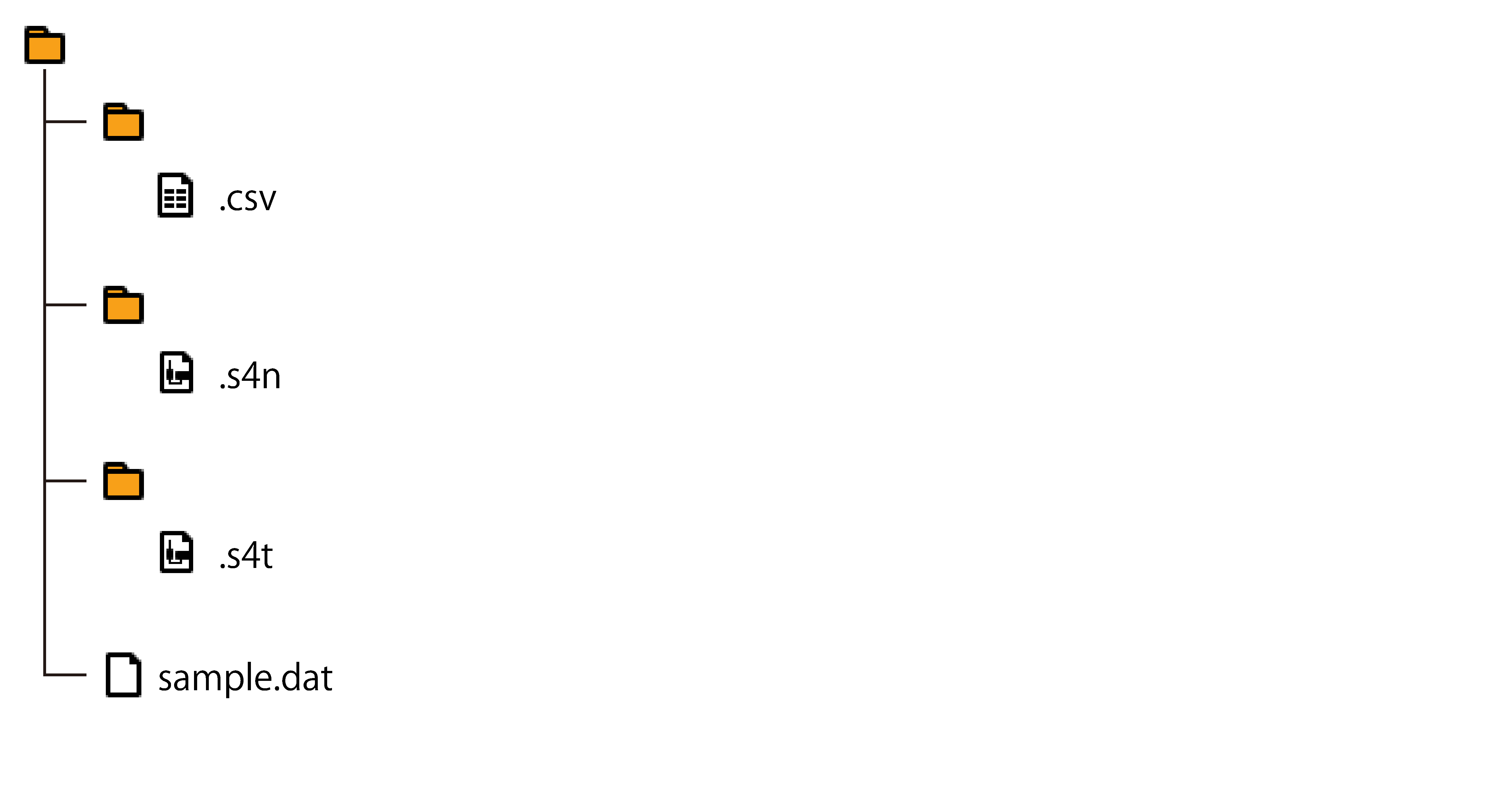
E-CON5 folder
exports folder
CSV files saved with the E-CON5 app.
sensors folder
Files containing custom sensor setup information created with the E-CON5 app.
setups folder
Setup files saved with the E-CON5 app.
This measurement result data file is created only when the number of measurement samples is extremely large.